Exploring Parametric Curves

By Rebecca L Adcock

 

 

 

Parametric equations are pairs of equations, usually in the form of “x=” and “y=”. The two equations together define the points of a graph in terms of a third parameter, usually “t”.

Let’s see what happens to the graphs when various coefficients are changed are a basic pair of equations. In the graph below the purple circle has coefficient ‘1’. Changing it to ‘2’ increases the size of the circle.

          

 

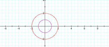
Graph 1

           

This graph gets a little more interesting. The purple and red circles are created when the constants of the cos and sin expressions are equal. The ellipses are created when they are unequal. When the constant for the sin expression is larger, the ellipse is longer along the y-axis. When the constant for cos is larger, the ellipse is longer along the x-axis.

Graph 2

 

Let’s stop a moment and think about what we are seeing. We are looking at graphs that represent the values that ‘solve’ the two equations. Let’s look at a cosine curve….

(purple)                     (red)

 

Graph 3

 

 

and a sine curve…..

 

(purple)                 (red)

 

Graph 4

 

We see curves that continually repeat along the x and y axes (in the example I’ve chosen). The extreme values of the curves never exceed 1 on the scale.

 

Review:

The sine and cosine functions are periodic. That means their pattern (and values) repeat over a period. Sine and cosine have a period of 2pi. Notice that the curves never get more than 1 unit away from the axis. This is the amplitude. We can change the amplitude by multiplying sine and cosine by some number.

 

Hey, wait a minute! We saw that happen in Graphs 1 and 2. When we multiplied sine and cosine by a number the circles and ellipses got bigger. We increased their amplitude. Notice another similarity. While the sine and cosine graphs are bounded by 1 (in our example) , the parametric equations are bounded also. We called that amplitude in our review. Our parametric equations are bounded all the way around, like they are contained in a rectangle.

 

Now that we’ve refreshed our memories on sine and cosine, let’s look at some more parametric equations and see what else we can learn.

 

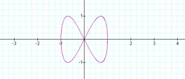
Notice in Graph 5 that although the value of ‘b’ is 2, the graph is contained with a ‘1 by 1’ area. (We didn’t change the amplitude.) There are two peaks on each side of the x-axis. Is that significant?

 

 

 

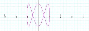
Now b=3 and the graph has changed so that there are 3 peaks above and below the x-axis.

 

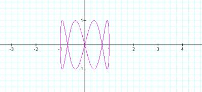
Four peaks and b=4…

b=4

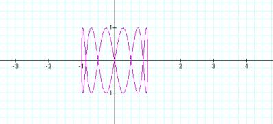
Six peaks and b=6…

 

If we increase the values of a and let b=1, here’s what we get….

 

 

Very similar to b> a . but oriented around the y-axis.

So what happens when a and b are greater than 1 and a not equal to b?

 

Wow! Change around 2 numbers and things changed completely. But look below where I change two numbers around and the graphs are very similar….

 

 

 

 

 

We’ve really seen the power of numbers here. Depending where in an expression you make a change, you can increase the size, orientation, and the appearance of a graph, sometimes in unexpected ways. So let’s do just a little more investigation and see what happens when we raise the cosine and sine functions to powers greater than 1.

 

If we look at this parametric pair where a=b and their value ranges from 1 to 2.5, we get this….

If we set a and b less than 0…..

Let’s see what happens when we increase to a power of 3….

That’s a big change from the line segments in the previous two graphs.

If we increase to a power of 4 and a and b both positive and negative ….

 

To a power of 5….

 

If we look back at this lesson we can see a wide range of curves that are all produced by cosine and sine expressions both singly and in parametric pairs. Singly, the curves are continuous, in pairs they are bounded.

 

 

Return