Assignment 10: Parametric Equations and Graphs

by

Tom Cooper

In many mathematics classes we study function where one variable depends on the value of another. Typically, we write y as a function of x and plot graphs in the xy-plane. However, x and y could both depend on a third variable t. This often happens in the real world where t is time and x and y both vary over time.

For example suppose that x = cos(t) and y = sin(t). For any given t, we get an ordered pair (x, y). For example when t = 0, we have x = cos(0) = 1 and y = sin(0) = 0,  or (x,y) = (1,0). We could generate lots of the points and plot them in the xy-plane.

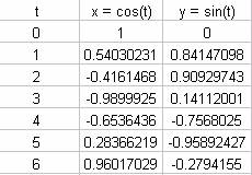
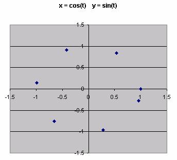
Powerful graphing software, such as Graphing Calculator, we can plot enough points to get a continuous curve. Since sin(t) and cos(t) are periodic, it is only necessary to run t from 0 to 2 Pi.

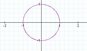
For this particular example, we get a circle with radius 1. Let's explore x = a cos(t) and y = b sin(t).

Here is a graph with 5 different sets of values.

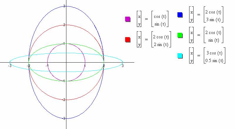
You should note that each graph is an ellipse. The parameters a and b control how far the ellipse stretched on the x and y axis respectively.  Explore these graphs here.

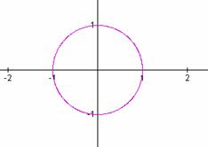
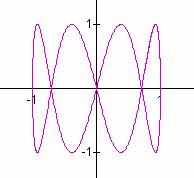
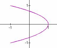
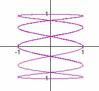
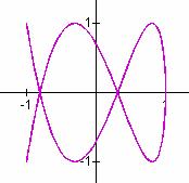
Now lets examine x = cos(t) and y = sin((a/b)t).  In order to get a complete picture, run t from 0 to .

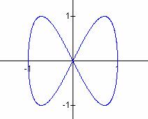
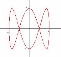
a/b = 1                                                             a/b = 2                                     a/b = 3

a/b = 4                                                 a/b = 1/2                                  a/b = 1/3

a/b = 1/4                                              a/b = 1/5                                  a/b = 1/6

a/b = 2/3                                              a/b = 2/5                      a/b = 3/4

a/b = 3/5                                              a/b = 5/7                      a/b = 5/6

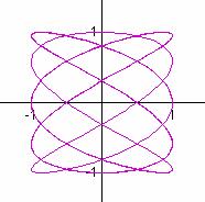
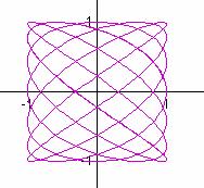
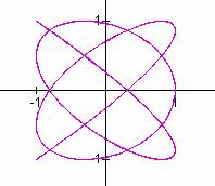
a/b = 3/2                                              a/b = 5/2                      a/b = 4/3

Do you detect any patterns? Explore these graphs here.

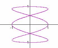
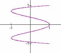
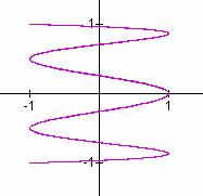
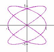
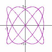
It seems that when b is odd, b tells the number of loops up the y-axis between -1 and 1, and a tells the number of loops along the x-axis between -1 and 1.

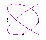
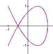
In these cases, the graphs are symmetric about each axis. When b is even, we get a "pretzel" shape which is symmetric about the x-axis, but no the y-axis.

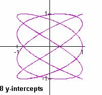
Also in the case when b is even, it seems that  b gives the number of y-intercepts.

a/b = 5/8

a/b = 7/12

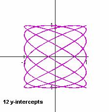
Does a tell anything?

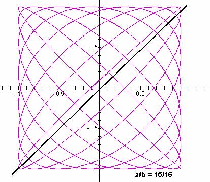
It seems to be the number of times that the black line crosses the purple above.

Now lets explore a different set of equations.

x(t) = a + t                    y(t) = b + kt

Let’s begin by fixing a = b = 1 and changing k.

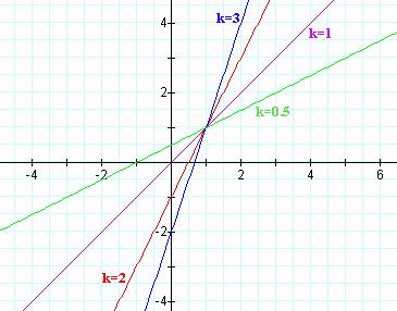
The above graph indicates that the graph is a line with slope k.

Let’s try a = 2, b = 3 and vary k.

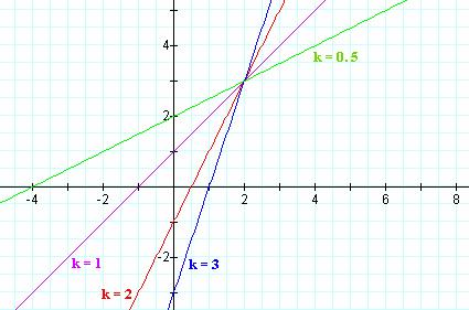
There are different y-intercepts, but we still have straight lines with slope k. More exploration with Graphing Calculator gives much evidence that all of the graphs will be straight lines with slope k.

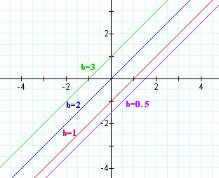
Let’s fix k and b at 1 and 2 respectively and manipulate a.

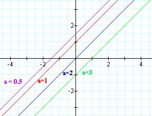
It seems that as a increases, the y-intercept decreases. Now let’s fix a = 2, k=1, and move b.

It seems that as b increases, the y-intercept increases.

It is actually easy to convert from x = a + t, y = b + kt  to a Cartesian formula.

If x = a + t, then t = x – a.

So y = b + kt = b + k(x – a) = kx + (b – ka).

Thus, the graph is indeed a line with slope k and y-intercept  b – ka.

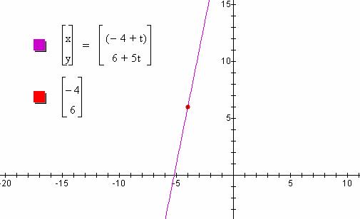
Now suppose that we want a set of parametric equations for a line with slope k passing through the point (m, n).

We must have x(t) = m + t and y(t) = n + kt. Then we have seen that k is the slope and (x(0), y(0)) = (m + 0, n + k(0)) = (m,n).

For example, a line with slope 5 passing through the point (-4, 6) would have equation x(t) = -4 + t and  y(t) = 6 + 5t.