Exploring Parabolas
by Kristina Dunbar, UGA
![]()
Explorations of the graph
In this exercise, we will be exploring parabolic graphs of the form y = ax2 + bx + c, where a, b, and c are rational numbers. In particular, we will examine what happens to the graph as we fix 2 of the values for a, b, or c, and vary the third.
We have split it up into three parts:
![]()
Let a vary while b and c remain fixed.
Example 1: Let b = 0 and c = 0.
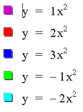
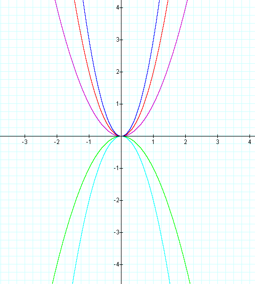
So, what's happening? The traditional graph of y = x2 is shown in purple. We have seen that increasing the value of the coefficient a narrows the parabola, and changing the sign of the coefficient a changes the direction of the parabola.
Example 2: Let b=1 and c=0 while still varying a.
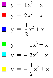
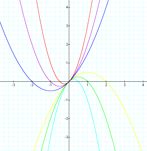
So, what is happening now? All of these parabolas still pass through the origin, but the bases of the parabolas have moved.
Example 3: Let a vary, b = -1, and c = 0.
Based on the picture above, I would expect it to look similar to Example 2, except that the graph will shift to the right for the upward-shaped parabolas and to the left for the parabolas facing down. Let's see if we're right.
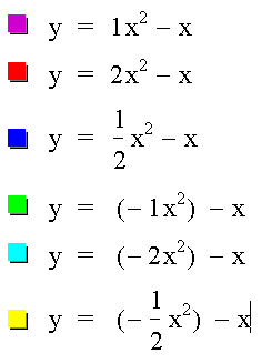
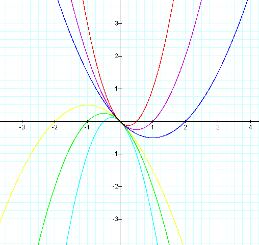
The graph did exactly what we expected it to do, based on our observations in the previous graph.
Example 4: Vary a and let b = 1 and c =1.
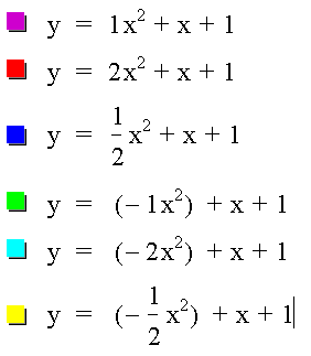
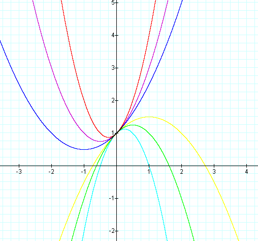
We see that the parabolas no longer go through the origin, but through the point (0,1) instead.
![]()
Return to my Home Page.
Return to my Assignment List.
Return to: Top varying a varying b varying c
![]()
Let b vary while a and c remain fixed.
Example 1: Let a = 0 and c = 0.
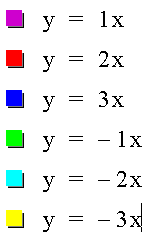
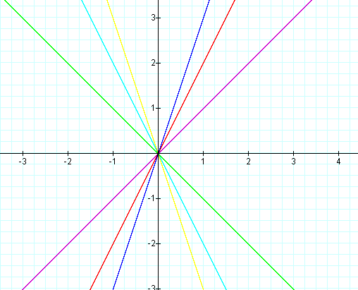
I don't think there is anything really surprising in the picture above. With both a and c equal to zero, we are left with a linear function. When b is positive, the line remains in quadrants I and III, the quadrants where both x and y have the same sign / direction. When b is negative, the line is in quadrants II and IV. Notice that these lines always go through the origin, and that when you increase b, the line gets steeper.
Example 2: Let a = 0 and c = 1.
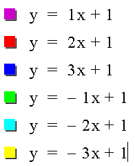
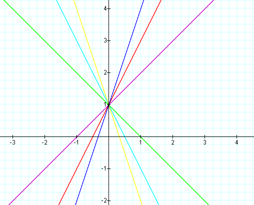
The graph looks exactly like the one above, except for the fact that it has shifted 1 unit in the positive direction. The graphs no longer go through the origin, but through the point (0,1). Also, notice that now the equations for the graphs are the normal linear equations of the form y = mx + b, where m is the slope and b is the y-intercept.
Example 3: Let a = 1 and c = 0.
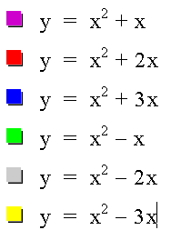
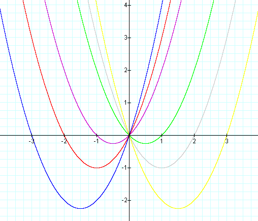
We now have a parabola again. Notice that the bases of the parabolas are all below the x-axis and that they still go through the origin. The graphs with positive values of b have shifted down and to the left, those with negative values of b have shifted down and to the right.
Example 4: Let a = 1 and c = 1.
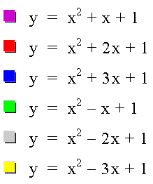
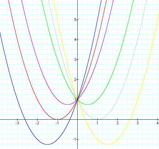
The graph looks like the one in Example 4, except for the fact that it has shifted up one unit and all parabolas go through the point (0,1).
![]()
Return to my Home Page.
Return to my Assignment List.
Return to: Top varying a varying b varying c
![]()
Let c vary while a and b remain fixed.
Example 1: Let a = 0 and b = 0.
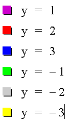
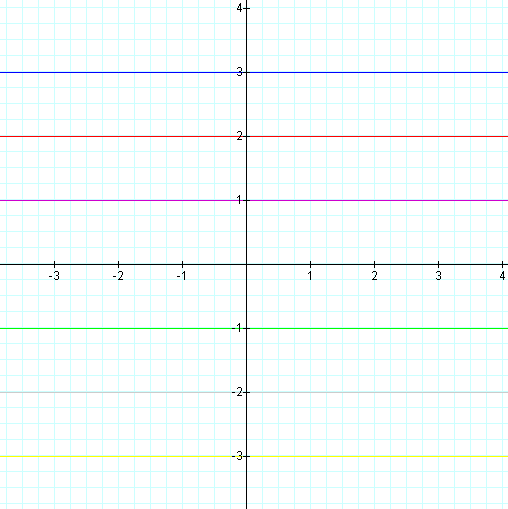
These are all horizontal lines crossing the y axis at the c value.
Example 2: Let a = 1 and b = 0.
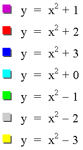
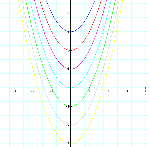
We have a normal parabola with the base of the parabola on the y-axis at the value of c.
Example 3: Let a = 0 and b = 1.
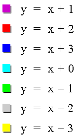
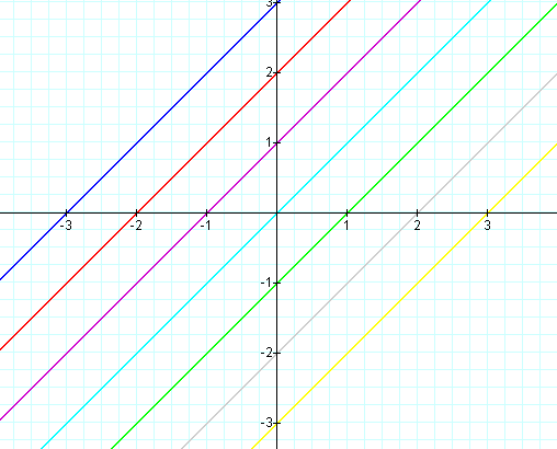
All of these graphs have a slope of 1 (the b value) and cross the y-axis at the c value.
Example 4: Let a = 1 and b = 1.
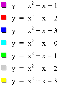
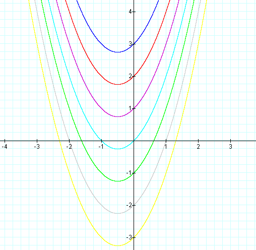
We have a series of parabolas whose bases are to the left of the y-axis and that cross the y-axis at the c value.
![]()
Return to my Home Page.
Return to my Assignment List.
Return to: Top varying a varying b varying c
![]()