Let's begin our discussion of quadratic equations by considering the following equation and its graph.
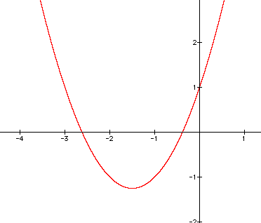
First, let's notice that the curve is a parabola. In ancient times the Greeks studied the parabola along with associated curves called Conics or Conic Sections. The properties of a parabola are very interesting as we shall see. In the above graph notice that the point (0,1). We shall now overlay several parabolas which will share that same point by choosing different values of bx. We may call the collection of curves a family related to the original quadratic equation.

The key feature to notice is that all the curves go through the same point (0,1) even though changing bx has the effect of horizontally shifting the curve parallel to the x-axis.
Now, recall that the solutions to a quadratic equation are called the roots or zeros. Simply, the solutions of a quadratic can be real numbers, complex numbers, or a combination of reals and complex. Graphically, if the curve intersects the x-axis then that intersection point is a real solution or root of the equation. However, if the curve does not touch or cross the x-axis then the root would be complex. As an example look where the following equations intersect the x-axis in the above graph. The yellow curve has one root at approximately (1.5, 0) and (2.5, 0).
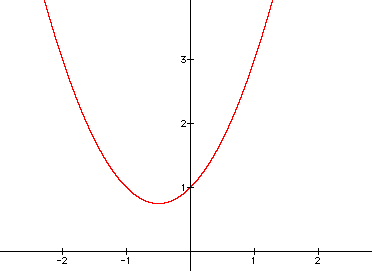
Now, to further our discussion, let's take a look at the locus of vertices of the family of curves. Think of the the locus as a collection of points and vertices as the bottom most point in all the above curves. Note,however, the vertex would be upper most point on the curve if the curve opens downward. In this graph we will make the family of curves on one color so see can see how the locus of vertices relates to the family.
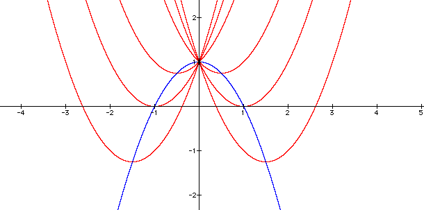
The above graph is telling us that the collection
of points which represent the vertices of each of the parabolas
traces the blue curve which is defined by the quadratic equation
![]() . As with the family of curves,
the blue curve also shares the point (0,1)!
. As with the family of curves,
the blue curve also shares the point (0,1)!
Notice, also, that the blue curve opens downward as opposed to the family of curves which all open upward. We, therefore, can conclude that if the first coefficient is positive the curve opens upward and if the coefficient is negative then it opens downward.
Now, returning to the roots of a quadratic equation, we will explore the bx term of the quadratic equation in more detail. We want to understand the relationship between this term and the roots of the original equation. On face value, one may think that the bx would not tell us about a solution of an equation which also includes the ax^2 and cx terms. Let's see what occurs when we fix the values of the two other terms and graph the bx term on the bx plane.
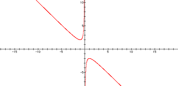
The bx plane is similar to plane except that we allow the bx term to be expressed on its own plane. A simple way to think of this is we are simply substituting the y-axis for the b-axis and graphing the quadratic equation by fixing the values of the two other terms. What we see above is a graph where the b-axis is an asymptote, that is, the curve will come very close to the b-axis but will never touch or cross the axis. When the x values are negative the curves lies in second quadrant. Likewise, when x values are positive the curve lies in the fourth quadrant.
Let's consider adding an other curve such as b = 3 to the graph. In this case the b = 3 relates to our original equation where the coefficient of b was 3. Where the curve of b = 3 intersects the red curve our points that tell us what the x values are. That is, the x values in the below graph are the x values of the original quadratic equation, i.e. the roots!
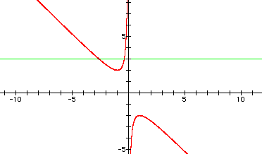
As a comparison, let's reproduce the original equation to convince ourselves that the roots are indeed the same. If you draw a line down from the rightmost intersection point to the x-axis you will see the x is approximately -2.5. Likewise, the below graph has a rightmost x-intercept at -2.5! Therefore, we could select different values of b on the bx plane and match the x values to the roots of a corresponding equation on the xy plane.