Using Graphing Calculator 3.2, we can explore the continuous sine curve expressed by the equation

By examining various graphs of:
for different values of a, b, and c, we are
able to see the specific impact these values have on our original
curve.
In order to explore the sine curve in terms of the coefficient a, we must examine a when b = 1 and c = 0 in our original equation. Let's first look at positive values of a. What happens to the corresponding graphs as the value of a changes?
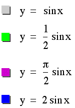 .
.
The original sine curve is represented by the gray line. Regardless of what value is chosen for our coefficient a, the intersections of this graph along the x-axis will remain x=0, x=pi, and x=2pi. By choosing different positive values of the coefficient a, we can see our original sine curve has changed only in amplitude, or height.
Now, what can we expect for negative values of a? Let's examine the following graphs:
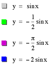

Again, amplitude of the original sine curve has changed, as we would expect. The intersections of this graph and the x-axis are still at x=0, x=pi, and x=2pi. The difference with a negative value of a however, is our sine curve now has a negative amplitude. In other words, our graphs are the same as when a was a positive value, but are now reflected across the x-axis.
To see a direct comparison between positive and negative values of a, click here.
Watch the animation of our sine curve as a
goes from -5 to 5. Notice how different
values of a change the amplitude of our sine curve.
See how the curve appears to be growing in height in the y direction.
For this exploration, we must assuming a=1 and c=0 to examine the effect the coefficient b will have on our original sine curve. Let's begin by exploring positive values of b. What happens to the corresponding graphs as the value of b changes?

The original sine curve is represented by the gray line. This time, different values of our coefficient result in different points of intersection at the x-axis. Are curves no longer intersect the x-axis at x=0, x=pi, and x=2pi. By choosing different positive values of the coefficient b, we can see our original sine curve has changed only in period, or the length of one cycle. In other words, the period for the sine curve to make one full osscilation is no longer from 0 to 2pi.
What happens when b has a negative value? Let's examine the following graphs:
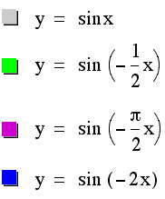

Again, the period of the original sine curve has changed here, as we would expect. The difference with a negative value of b however, is our sine curves have the same period as the positive values of b above, but now they are reflected across the x-axis.
For a direct comparison between positive and negative values of b, click here.
Watch the animation of our sine curve as b
goes from -5 to 5. Notice how different
values of b change the period of our sine curve.
See how the curve appears to be contracting and expanding along
the x-axis.
In this case, we are assuming a = 1 and b = 1 in order to demonstrate the affect the coefficient c will have on our sine curve. First, let's look at the graphs generated for positive values of c. What happens to the corresponding graphs as the value of c changes?
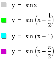

The original sine curve is again represented by the gray line. This time, different values of our coefficient result in different positions of our graph along the x-axis. Are curves no longer intersect the x-axis at x=0, x=pi, and x=2pi, but the do have the same period. By choosing different positive values of the coefficient c, we can see our original sine curve has changed only in phase. In other words, the period for the sine curve to make one full osscilation is still an inverval length of 0 to 2pi like the original curve, but now all of the graphs have all been shifted to the left.
What happens when c has a negative value? Let's examine the following graphs:
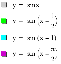

Again, the phase of the original sine curve has changed here, as we would expect. The difference with a negative value of c however, is that our sine curves have been shifted to the right this time. They all still have the same period as the positive values of c above, but now they have moved in the other direction along the the x-axis.
For a direct comparison between positive and negative values of c, click here.
Watch the animation of our sine curve as c
goes from -5 to 5. Notice how different
values of c change the phase of our sine curve.
See how our curve appears to be moving back and forth along the
x-axis.
Return
to Class Page