By using Graphing Calculator 3.2, we can explore different types of polar equations. A polar equation is the equation of a curve expressed in polar coordinates.
Let's investigate graphs of the following equation, for different values of a, b, and k. Please note that our value for theta must be between 0 and 2pi inorder for the graphs to be closed. See what happens to the graph of the equation, if theta is defined over different intervals.
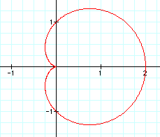
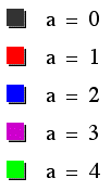
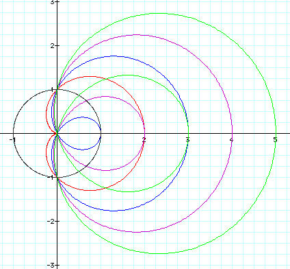
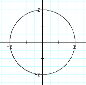
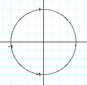
To investigate different values of a, let b=1 and k=1. Let's see what happens to our graph when a changes.
 |
 |
As the value of a gets larger, our graph looks more and more like a circle.
View the animation as the value of a
goes from 0 to 5.
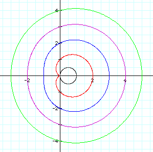
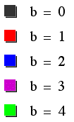
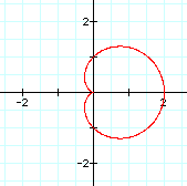
To investigate different values of b, let a=1 and k=1. Let's see what happens to our graph when b changes.
 |
 |
It seems as though with increasing values of b, the loops on our graphs get larger. Notice when b is greater than or equal to 2, the graph actually has two loops. One on the inside, and one on the outside.
View the animation as the value of b
goes from 0 to 10.
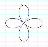
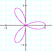
To investigate different values of k, let a=1 and b=1. Let's see what happens to our graph when k changes. It is easier to view the effect of a changing k value if these graphs are viewed individually.
|
|
|
|
|
|
 |
 |
 |
 |
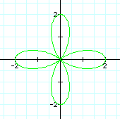 |
It seems as though the value of k determines how many "pedals" are graphed. For example, the graph when k=4 above shows four pedals around the origin. These graphs represent what is known as the "n-leaf rose," where n is the value of k. These graphs are drawn when a=b (in this case, both equal 1), and k is an integer.
View the animation as the value of k goes from 0 to 25 and watch as more "pedals" are generated.
Watch what happens when the values of a, b, and k all change together from 0
to 10. See how the "n-leaf rose"
is generated this way.
Let's compare our previous findings for k when a=0 and b=1. So, our equation now looks like:
Let's now explore this new equation for different values of k and compare the results to the graphs above.
|
|
|
|
|
|
 |
 |
 |
 |
 |
Immediately, we notice the domain and range of our graphs have changed. The graphs generated by this new equation fall between -1 and 1 on the x-axis, and -1 and 1 on the y-axis.
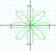
Also, we see other variations between the number and shape of the pedals of this new graph. Here, k does not always represent the number of pedals we are going to have in our rose. When k is even, there are 2k pedals graphed. For example when k=4, 8 pedals are graphed as shown above. So n=2k for our "n-leaf rose."
When k is odd, however, it seems to follow the examples from our original equation. So when k is odd, k directly represents the number of pedals graphed. As shown for k=3, there are three pedals graphed. When k is odd, n=k for our "n-leaf rose." Does this always work for odd and even values of k? Let's look at more values of k to find out.
View the animation as the value of k goes from 0 to 25 for this new equation. Can you see how this animation is different from the one above?
Watch what happens when the values of b, and k all change together from 0 to 10 for our new equation. See how the "n-leaf rose"
is generated this way. How is this different from the animation
above when b, k, and a changed together?
Let's look at the graphs of this new equation as the values of a, b, and k change. Our equation is now:
How do you think our graphs would change over the same interval for theta? Click to see an investigation of our new equation.