
A cycloid is the locus of points on a circle that rolls along a line. To understand what this means, click HERE to look at the GSP animation of the image below. (Here the circle has been moving towards the left and the point has been moving counterclockwise).
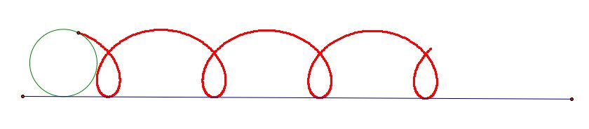
When you are playing with the GSP animation, try changing the speed of the point on the circle as well as the point on the line. This will change the appearance of the cycloid and you can see that the locus can take on many interesting shapes.
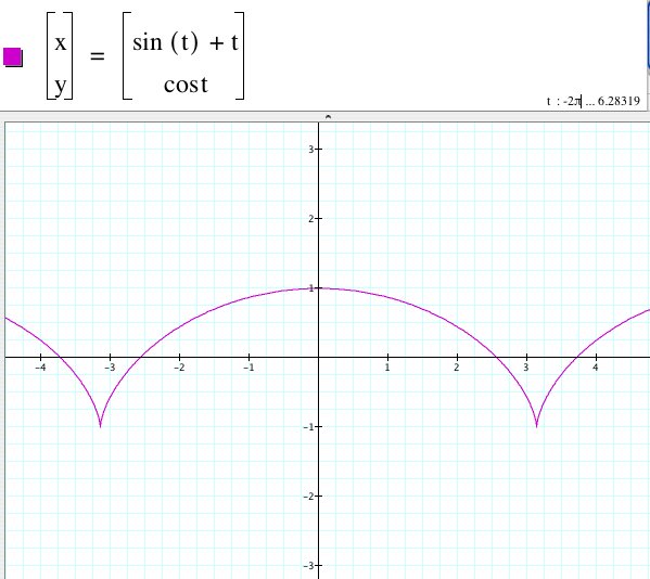
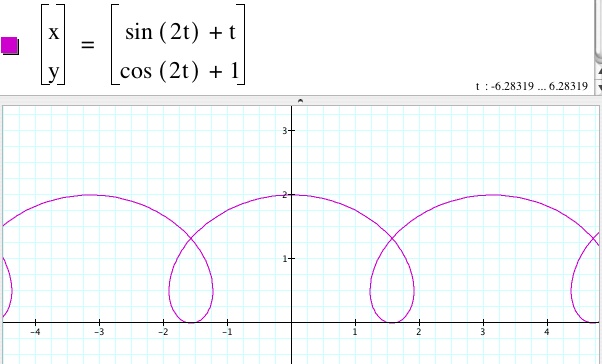
The challenge is to try to come up with parametric equations that can model the cycloid. In order to do this, I started with my prior knowledge of parametric equations. I knew that x = sin(t) and y = cos(t) gave me a circle of radius 1 centered at the origin. So what I needed to do was determine how to get this circle to "move" like it has in GSP. To do this, I determined that I would have to change my x equation. It occured to me that I would want the x to move horizontally, so that could be achieved my adding a t to the original equation. When I did this, my equations gave me the picture below.
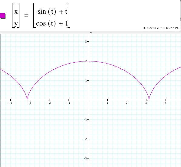
Already this was closer to what I wanted! But how was I suppose to get the loops? And if I wanted the cycloid to be rolling along the x-axis, how could I achieve that? Firstly, I knew that if I added 1 to my y-equation, that this would move the center of my circle vertically one unit. By doing this, I was able to get the cycloid on the x-axis.
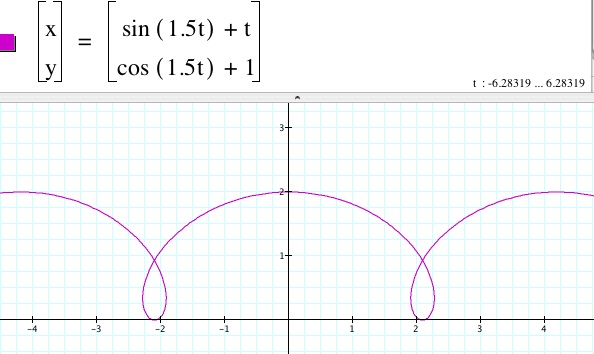
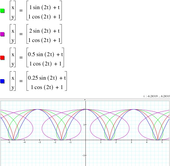
So the last step was for me to figure out how to get the loops. I knew from my GSP animation that the loops were related to the speed at which the points were traveling. In fact, I determined that the speed of the point on the circle had to be moving faster than the point on the line. Since the + t in the x-equation was controlling the horizontal movement, and its coefficient was now a 1, I decided that I would have to change the argument of the sine and cosine functions since these functions controlled the circular motion. I experimented with different values, but kept them all greater than 1, and saw that I could make my loop as fat or thin as I wanted. Below are a couple of examples.
 |
 |
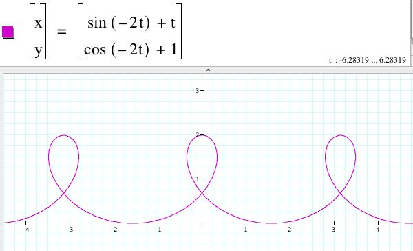
Now the coefficient for the sine and cosine functions could not have been just any number. In my investigation, I determined that the sine and cosine functions had to have the same coefficient. If the coefficient were positive, as above, the loops would be facing down. If the coefficients were negative, the loops would be facing up and the graph would be transformed horizontally so that a loop would be on the y-axis.
Why did this happen? The sketch below shows what happens from 0 to 2 pi.
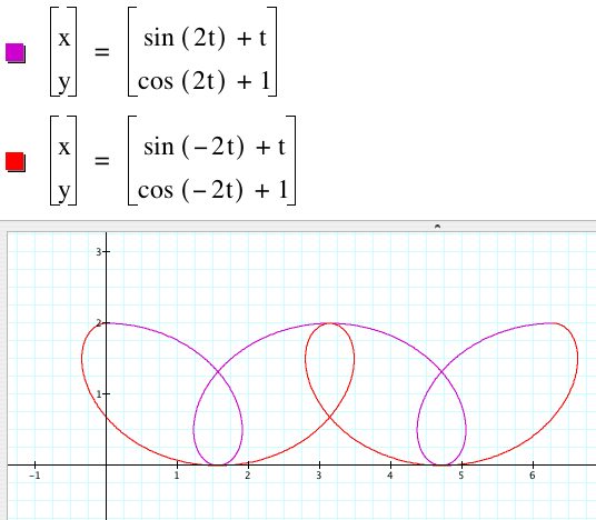
Notice that the direction of the loop has to do with the angle. When the argument is positive, as in the purple curve, the value of x will be increasing initially because the sine function is increasing in the first quadrant. Conversely, when the argument is negative, the value of x will be decreasing initially since the sine function is decreasing while it moves from 0 to negative 2 pi. Investigating this phenomenon on Graphing Calculator also may be helpful.
After having investigating this part of my parametric equation, I wanted to see if I could generalize the equations more and determine how to control all aspects of the loops. The general equations that I used were as follows:
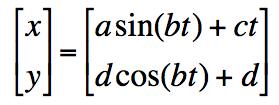
So what do each of these parameters control? Here is my list...
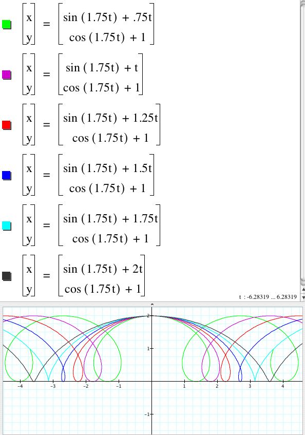
a: Controls what I call the "fattness of the loop. Basically, as a increases, the loop becomes wider, but they stay tangent at the same location. If a < 0 the loops will change orientation. If 0 < a < 1 (and c = 1), the loops disappear and a determines how "pointed" the graph becomes.
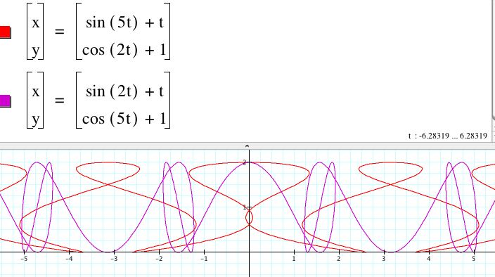
b: Controls the distance between the loops or the number of loops in the interval. When b > 0, the loops will face down, when b = 0 the graph is a line, and when b > 0 the loops will face up. (More discussion of this can be seen above). The parameter is the same in both equations so that the loops will be vertical. During my investigation I saw that when the coefficients were not equal, the loops seemes to slant. Under further study, I saw that when the coefficients differed by a significant amount, the loops disappeared all together! A complete discussion of this phenomenon is beyond the scope of this investigation, but I would encourage you to play with these parameters on your own. (Here are a couple of files to get you started; sine large, cosine large).
c: Controls the points of tangency for the loops. As c increases, the closest points of tangency move farther away from the origin. This parameter also controls the "fattness" of the loops. When c is greater than or equal to a, there will be no loops and c will control the how pointed the graph becomes. Hence, c acts very much like a and the two react with each other.
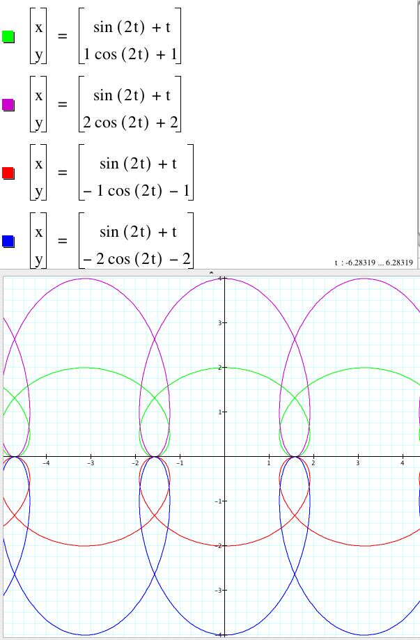
d: Controls what I call the "center" of the graph. In fact, it controls the amplitude of the loops. The reason that the d needs to be added on to the end is so that the points of tangency will always be on the x-axis. If d < 0, the graph is reflected across the x-axis.
There is much more to discover with these equations and it would be interesting to try to determine if there is a physical representation of the graphs beyond the point on the circle. But I will leave this up to you! Happy investigating!