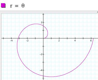
Polar coordinates allow us to explore graphs in new and exciting ways. Unlike the Cartesian coordinate system, which used lengths as their basis, the polar coordinate system uses radius and angle measure. Hence, when creating a function, we have r = radius as the dependent variable and theta = angle as the independent variable. One of the most basic equations, which may help you understand what is going on, can be seen below with theta defined from zero to 2 pi.
While I was looking at several polar equations, I noticed that there were certain ones that would give me conic sections. In this investigation, I will show you which equations gave me these graphs and try to explain how you can change the equations to get the conic section of your choice.
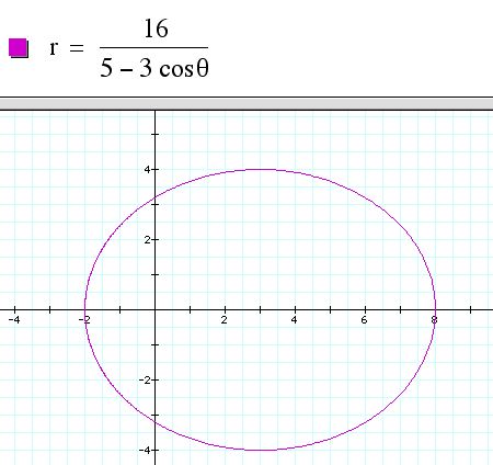
First let's look at an ellipse with center (3,0), a horizontal major axis of 10 units and a vertical minor axis of 8 units.
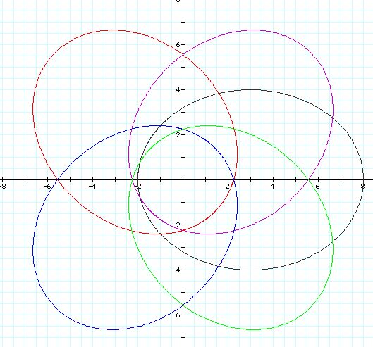
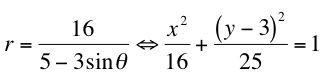
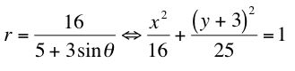
Now let's see how to rotate this ellipse 90, 180, and 270 degrees. This can be done quite easily with a change of sine to cosine or a change from subtraction to addition or a combination of both.

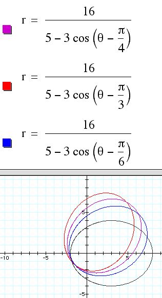
What about rotations of 30, 45, 60, etc.?
Any of these rotations can then be moved into the second, third, or fourth quadrant by replacing the minus cosine by minus sine (135 degrees), by plus cosine (225 degrees), or by plus sine (315 degrees).
So I wondered why all of this was happening. To figure it out, I changed my inital polar equation into rectangular coordinates. When changing polar into rectangular, you use
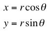
Hence, x^2 + y^2 = r^2. Furthermore,
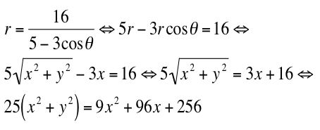
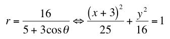
But this equation can be put into the form of an ellipse by completing the square. Thus,
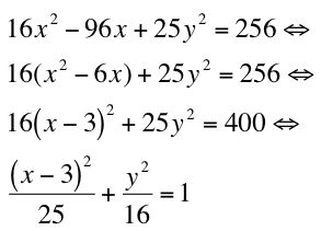
which is precisely an ellipse with center (3,0), a horizontal major axis of 10 units and a vertical minor axis of 8 units. So why did this ellipse move the way it did with the changing of sine and/or the negative sign? Well, if you go through similar calculations, it is easy to see the the following equations are equivalent:
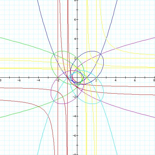
So then I wanted to see what would happen if I used both cosine and sine in the equation at one time. To do this, I started with a pretty basic equation and went from there. I began with the equation and graph

So it looked like this equation would give rise to a hyperbola. To investigate this further, I first used Graphing Calculator and changed the coefficents for the sine and cosine function as well as the other constants. The general equation that I worked from was
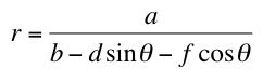 .
.Initially, a = b = d = f = 1. I then varied each parameter individually to see how it would change my graph. The following is a description of what I found:
a: Controls the asyptotes and intercepts. The vertical asymptote is x = -a, the horizontal asymptote is y = -a, the y-intercepts is (0,-a/2) and the x-intercept is (-a/2,0).
b: Controls the type of conic section that is graphed. When 0 < |b| < sqrt(2), the graph is a hyperbola and when |b| > sqrt(2), the graph is an ellipse. When b = 0, the graph is a line y = -x -1 and when b = sqrt(2), the graph is a parabola with directrix y = x and vertex (-0.25,-0.25).
a & b: If b = sqrt(2) and a varies, the parabola's vertex will always be at the point (-a/4,-a/4), and the directrix will remain y = x. When a > 0 the parabola opens up and when a < 0, the parabola opens down. If b = 0, Similarly, the equation of the line will be y = -x - a. If b is another value, the conic form, intercepts, and asymptotes will follow the rules above.
d: Controller of the vertical asymptote (x = -1/d) and effects the conic form as well as the horizontal asymptote. When d = 0, the conic is a parabola with equation y^2 = 2x + 1. When 0 < d < 1, there will be a slant asymptote with a positive slope which will be approaching the vertical asymptote x = -1 which occurs when d = 1. When d > 1, the slant asymptote will have a negative slope approaching 0 as d increases.
f: Controller of the horizontal asymptote (y = -1/f) and effects the conic form as well as the vertical asymptote. When f = 0, the conic is a parabola with equation x^2 = 2y + 1. When 0 < f < 1, there will be a slant asymptote with a positive slope approaching the horizontal asymptote y = -1 which occurs when f = 1. When f > 1, the slant asymptote will have a negative slope approaching 0 as f increases.
To see how d and f interact with a and b, it is fun to play with the Graphing Calculator, but the rules above will apply and interact accordingly. But its one thing to play with the graphs, and another to see what happens with the equation. So what I decided to do next was to change the polar equation to rectangular coordinates.
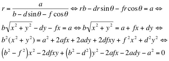
Notice that this is the general equation for a conic section. Furthermore, to determine the conic form, we look at A^2 - 4BC. In this case we have the following:
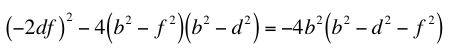
This means that our conic form with depend completely on the relationship between b, d, and f. Specifically, if b^2 - d^2 - f^2 < 0, then we will have a hyperbola, if it is positive, we will have an ellipse or circle, and if it equals zero, we will have a parabola.
So as you can see, polar equations have a wealth of information and are fun to play with. I would encourage you to use Graphing Calculator to see what kind of great pictures you can come up with.