---

Michael Thomason's final assignment.

---

Bouncing Barney

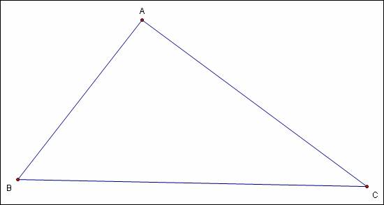
Prompt: Barney is in the triangular room shown here. He walks from a point on BC parallel to AC. When he reaches AB, he turns and walks parallel to BC. When he reaches AC, he turns and walks parallel to AB. Prove that Barney will eventually return to his starting point. How many times will Barney reach a wall before returning to his starting point? Explore and discuss for various starting points on line BC, including points exterior to segment BC. Discuss and prove any mathematical conjectures you find in the situation.

First I’ll draw and label Barney’s room:

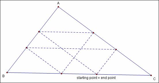
I have selected an arbitrary point for Barney to start his bouncing, and it turns out that he returns there after hitting five walls, with his sixth wall hit being at his starting point. Was I just lucky in my selection of a starting point? Click here to see an animation for different starting points along .

Does Barney always return to his starting point? Looking at the animation is pretty convincing, but here is some more evidence:

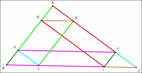
Congruent segments are colored similarly. For example, segment is congruent and parallel to . The distance covered by Barney’s path is equal to the perimeter of the room, triangle ABC.

What if Barney starts at a point on the continuation of that is outside the triangle? Let’s see:

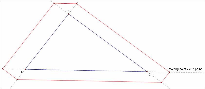
Once again, Barney ends up at his starting point regardless of the starting points location along .

Let’s look at this special case:

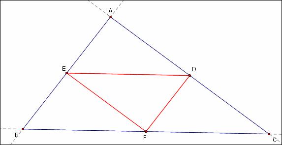
Let F, Barney’s starting point, be equal to the midpoint of .Barney still ends up where he started, but this time he only hits two walls before stopping at the third.

Claim: Triangle EBF is similar to triangle ABC.

Proof: || , , and EBF and ABC have the same angles and are therefore similar.

By similar proof: Triangles AED and DEF are similar to triangle ABC too.

So, since F is the midpoint of and the above mentioned triangles are all similar, E and D are the midpoints of their respective sides and triangle DEF is the medial triangle for triangle ABC .

---

Multiple Solutions
Prompt: Find as many solutions as possible for A, B, and C that satisfy both equations:
ABC = 4
3A + 2B - C = 3.
What observations can you make about your results?

The following was exported from this Maple worksheet. Open it and click and drag the three-dimensional plots to get a better idea of what’s going on.

First I'll graph .

> restart:with(plots):
a:=4;b:=15;
implicitplot3d(x*y*z=4,x=-a..a,y=-a..a,z=-a..a,grid=[b,b,b],axes=normal,style=patchcontour);

Warning, the name changecoords has been redefined




 
 
 
 
 

Now here's .

> implicitplot3d(3*x+2*y-z=3,x=-a..a,y=-a..a,z=-a..a,grid=[b,b,b],axes=normal,style=patchnogrid);

Now I will intersect the graphs and graph that intersection along the xy plane.

> z:=solve(x*y*z=4,z);
solve(3*x+2*y-z=3,y);
y[1]:=x->1/4/x*(-3*x^2+3*x+sqrt(9*x^4-18*x^3+9*x^2+32*x));
y[2]:=x->1/4/x*(-3*x^2+3*x-sqrt(9*x^4-18*x^3+9*x^2+32*x));

> plot([y[1](x),y[2](x)],x=-6..6,y=-6..6,scaling=constrained,color=red);

This graph looks a lot like the contour lines in the 3d plot of , but the plane is not parallel to the xy plane as one can see from its graph, so the graph of their intersections is skewed a little bit to correspond to the slope of the plane.

Here's another system of equations, their graphs, and the graph of their intersections:

> restart:
with(plots):
a:=5;b:=10;
x^2*y*z=4;implicitplot3d(x^2*y*z=4,x=-a..a,y=-a..a,z=-a..a,grid=[b,b,b],axes=normal,style=patchcontour);
2*x-y+3*z=7;implicitplot3d(2*x-y+3*z=7,x=-a..a,y=-a..a,z=-a..a,grid=[b,b,b],axes=normal,style=patchnogrid);

Warning, the name changecoords has been redefined




 
 
 
 
 

> z:=solve(x^2*y*z=4,z);
solve(2*x-y+3*z=7,y);
y[1]:=x->(x^2-7/2*x+1/2*sqrt(4*x^4-28*x^3+49*x^2+48))/x;
y[2]:=x->(x^2-7/2*x-1/2*sqrt(4*x^4-28*x^3+49*x^2+48))/x;
plot([y[1](x),y[2](x)],x=-6..6,y=-6..6,scaling=constrained,color=red);

---

Stamp Problem
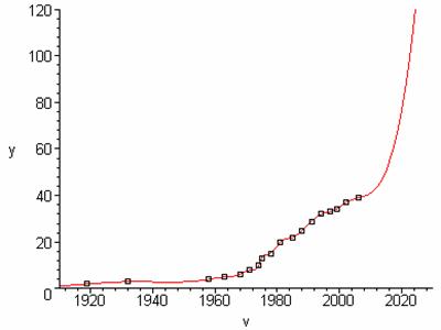
Prompt: Consider the Stamp Problem in Assignment 12. Update the data to include the price increases for a first class letter through January 2006 -- when the price will become 39 cents. (Recent increases were 33 cents in 1997, 34 cents in 1999, and 37 cents in 2002.)
Here is the stamp data and a plot of the points:

Stamp Price

year	rate(in cents)
1919	2
1932	3
1958	4
1963	5
1968	6
1971	8
1974	10
1975	13
1978	15
1981	20
1985	22
1988	25
1991	29
1994	32
1997	33
1999	34
2002	37
2006	39

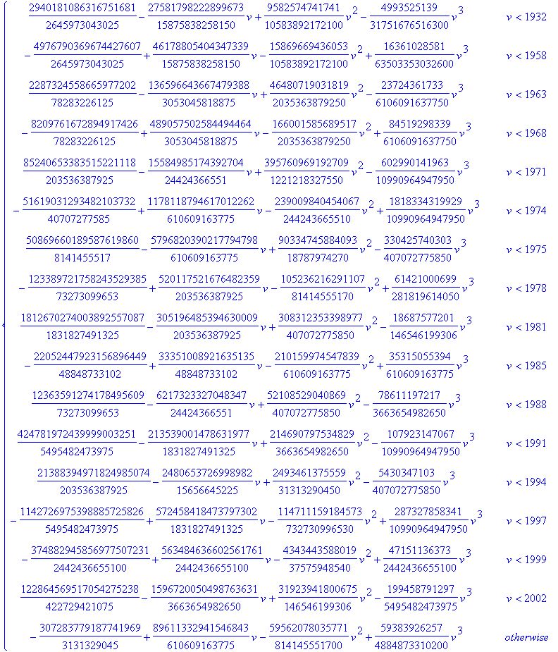
I used this Maple worksheet to create a function that fits the data above and a graph of that function. Click here to see the piecewise function. Here is the graph along with the stamp data:

When will the cost of a first class postage stamp reach $1.00?
To answer this, I used Maple’s fsolve command to find that the cost of a postage stamp will equal $1.00 (100 cents) sometime in the year 2022.

When will the cost be 74 cents?
Sometime in the year 2019.

How soon should we expect the next increase?
The function I used to model the data continues to grow even more rapidly after 2006, so it would suggest postage increases every year from now on. This is not very realistic, but it does convey the point that postage rates are increasing even more quickly now than before, and unless some other variable changes (inflation, gas prices, the invention of a cheaper method of mail delivery, et cetera), the trend will continue.

In 1996, the analysis of stamp data historically seemed to show that the postage doubled every 10 years approximately. The cost in 2006 would seem to argue that pattern is no longer valid. Is there evidence to show a change in the growth pattern? Or, was the 'doubles every ten years' just a bad model?
Doubling the stamp price from a given year and comparing it to the price ten years later should produce approximately the same value if the ‘doubles every ten years’ model is correct.

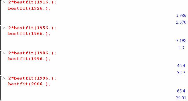
The doubling model seems roughly accurate at first, but as time progresses, it becomes less accurate. The cost in 2006 does indeed argue that the pattern is no longer valid.

---

Return to my main page.

---