Looking at Distance Equations

by Margaret Trandel

 

We have studied the distance formula and use it to calculate the distance between any two points. To review, the distance formula =

D =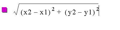

 

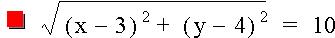
For instance, if we wanted to calculate the distance between the two points, (3, 4) and (-5, -2) we would simply plug the values into the formula and see that the total distance is 10 units.

D=

 

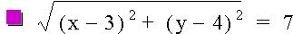
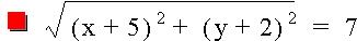
But what happens when we plug the coordinates above into two separate distance formulas and create distance equations instead of simply a distance formula. Let's take a look:

D1=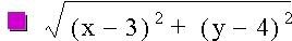             D2=

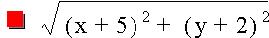
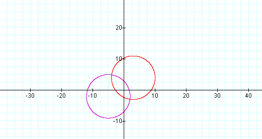
Graph:

 

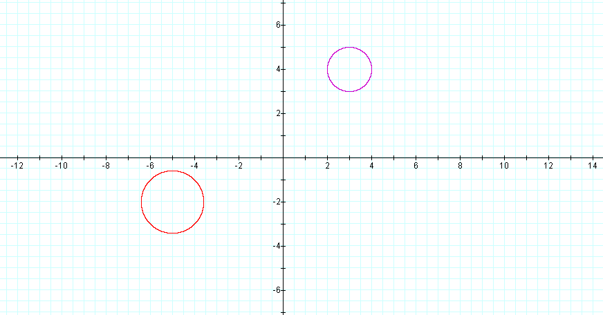
Did you expect the graph above? Why did we get circles? Let's take a look below and see what happens when D1 and D2 are replaced with constant values.

 

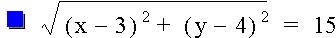
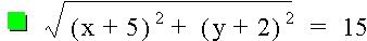
Setting Distance Equations Equal to Non-Zero Constants

Now let's investigate to see what happens when we adjust one side of the equation to a non-zero constant. As you can see from the graphs below, we end up with circles with varying radii, depending on the value on the right side of the equation.

 

 

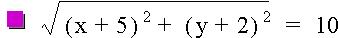
Below you'll find the graph:

 

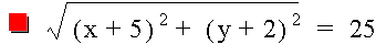
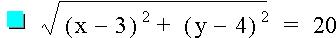
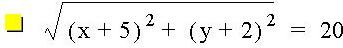
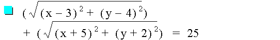
What happens when we change the constant to a larger value, such as 25?

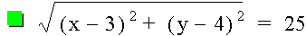
Did you anticipate the graph below? This was easier to predict than the behavior of the first graph because we knew what to expect.

 

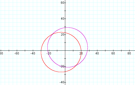
If we graph several equations using the same points but different constant values on the same graph we can see even more clearly that as the constant becomes larger so does the circle, and the center points remain the same.

 

 

Graph:

 

 

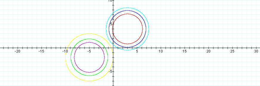
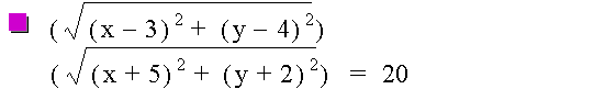
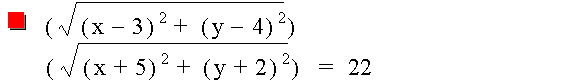
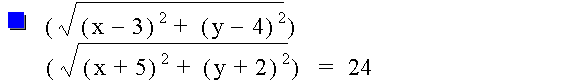
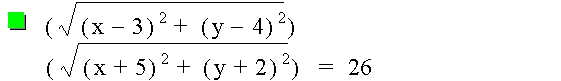
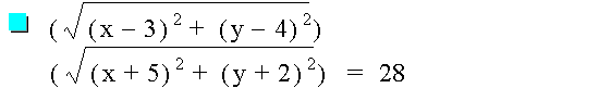
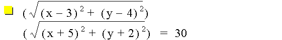
Exploring the Sums of Distance Equations

 

The equation below is a sample of two distance equations added together to equal a constant.

 

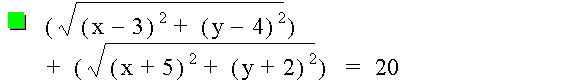
As we did in the last exercise, let's look at several equations and then graph them on the same set of axes.

 

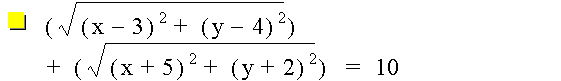
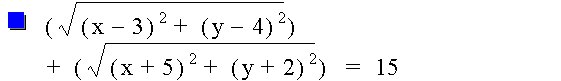
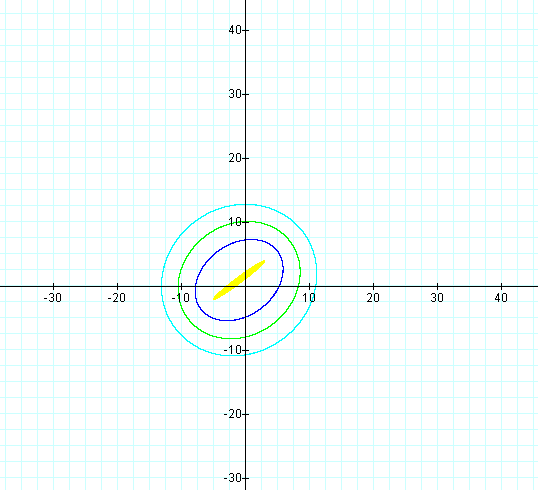
Is this what you expected? I was surprised! As the constant on the right side of the equation becomes larger, the figure becomes more and more circular.

 

The Product of Distance Equations

 

We shouldn't consider the sums of these distance formulas and ignore what happens with the product. Are you curious? Let's now try multiplying the same distance equations and note the graph.

 

Graph:

 

 

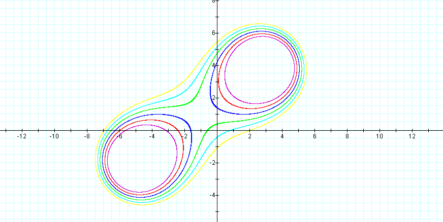
These ovals were first noted by Cassini and are called Cassinian Ovals. If you're interested, here's a web page that tells you more about Cassini Ovals.

 

Lemniscates

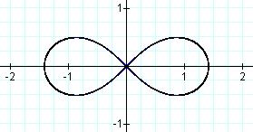
Let's do another investigation where we continue our look at products, but adjust our given points to (-a,0) and (a,0). Let's try a distance graph using (-3,0) and (3,0) as our assignment suggests, and set the right side equal to the square of +-3, which is 9.

Graph:

 

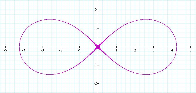
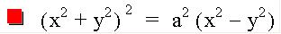
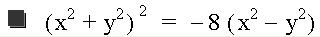
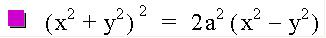
I did not expect this, did you? I did a little reading and found out there is a particular name for this graph. It is called the Lemniscate of Bernouilli. To review, the equation is the product of our distance equations Let's try to write this in general form, by first replacing the constants with variables and squaring both sides.

Simplifying gives us the following result:

 

 

Varying "a"

It's fun to vary a and see what happens to the graph.

 

 

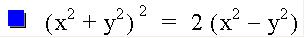
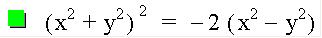
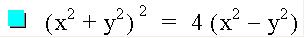
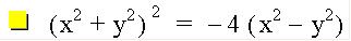
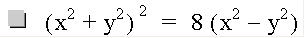
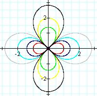
This is my favorite graph so far! Who would have thought that we could start with distance equations, do a little manipulation and end up with such a pretty graph! Note that with the negative coefficients we get the vertical petals.

 

 

Polar Form

Remember, to convert an equation in x and y to polar form we use x=rcos* and y=rsin*

In this particular instance we also need to use the trig identities of (sin*)squared plus (cos*)squared equals one and cos2*equals (cos*)squared minus (sin*) squared where * equals the angle measure.

Let's substitute these values in and manipulate the equation algebraically for a while. If we don't make any mathematical errors, our resulting graph should be a lemniscate. Let's try. Below I use theta to represent the angle measure.

 

 

 

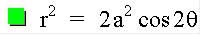
The Polar equation form graphed how I hoped it would -another Lemniscate.

 

I hope you have enjoyed this introductory investigation into distance equations and the variety of graphs which result when we use different operations and change constant values. To extend this investigation further, think about why the graphs behave as they do, and e-mail me. Thanks for participating!

Ms. Trandel