---

Stamps Over the Years

Assignment 12 – Diana May

---

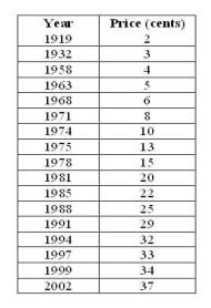
In 2006, the price of first class stamps rose from $0.37 to $0.39.   An increase in stamp prices rarely surprises people in modern times, but looking back at how the price of stamps has changed can be quite surprising.  We'll look at how the price of stamps has changed from 1919-2002 and try to develop a model to predict the price of stamps in the future.

Data

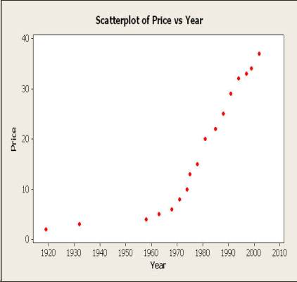
From looking at the graph, we see that the relationship between the price of stamps and the year is not quite linear.  When we attempt to fit a linear regression line to this data, we get the following regression analysis:

The regression equation is

Price = - 914 + 0.472 Year

S = 6.25393 R-Sq = 75.7% R-Sq(adj) = 74.1%

Analysis of Variance

Source	DF	SS	MS	F	P
Regression	1	1825.6	1825.6	46.68	0.000
Residual Error	15	586.7	39.1
Total	16	2412.2

Noticing that this linear regression equation is not a good fit (R² = 0.757); we can attempt to correct for this by transforming the data.  Performing a 1/y transformation on the data, we get the following regression:

The regression equation is

1/y = 11.2 - 0.00561 Year

S = 0.0355551 R-Sq = 93.2% R-Sq(adj) = 92.7%

Analysis of Variance

Source	DF	SS	MS	F	P
Regression	1	0.25823	0.25823	204.27	0.000
Residual Error	15	0.01896	0.00126
Total	16	0.27720

This regression appears to be a better fit (R² = 0.932); however, even with this transformation, we can see from the graph that the relationship is still not quite linear.  It seems that the transformation has distorted parts of the data that initially appeared to follow a more linear trend. Also, this regression becomes problematic when attempting to make predictions about future stamp prices, as we’ll see later.

---

In Context

One thing you might notice is that the trend seems linear up until about 1968 and then the price increases at higher linear rate.  It might be beneficial to consider what happened with the United States Postal Service around that time.  The Postal Service Act, signed on February 20, 1792 by George Washington, created the United States Post Office Department as a cabinet department, headed by the United States Postmaster General.  In 1970, the Postal Reorganization Act abolished the United States Post Office Department and created the United States Postal Service, a corporation that acted independently of tax dollars and that had an official monopoly on mail service in the United States.  

Perhaps if we group prices of stamps into two different categories, based on before or after the Postal Reorganization Act, we might find more suitable regression lines for the data.

---

Conducting a separate regression on the pre-1972 data set, we obtain the following regression:

The regression equation is

Price A = - 134 + 0.0708 Year A

S = 0.537473 R-Sq = 91.3% R-Sq(adj) = 88.4%

Analysis of Variance

Source	DF	SS	MS	F	P
Regression	1	9.1334	9.1334	31.62	0.011
Residual Error	3	0.8666	0.2889
Total	4	10.0000

This regression seems to be a good fit to the smaller data set (pre-1972), with an R² value of 0.913. The slope of the regression equation, 0.0708, tells us that each year, the price of the stamp would be predicted to increase 0.0708 cents. That means that it would take about 14 years for the price to increase by one cent!

---

For the post-1972 group, we get the following regression:

The regression equation is

Price B = - 1858 + 0.947 Year B

S = 1.16083 R-Sq = 98.8% R-Sq(adj) = 98.7%

Analysis of Variance

Source	DF	SS	MS	F	P
Regression	1	1092.2	1092.2	810.52	0.000
Residual Error	10	13.5	1.3
Total	11	1105.7

This separate line does an excellent job fitting the data, with an R² value of 0.988. Also, the regression equation has a slope of 0.947, which means that each year, this model predicts the price of a stamp will increase by 0.947 cents.

---

Let’s see how our different regression equations predict future prices of stamps. The years of interest displayed here are when one of the regression equations predicts the price of a stamp to be approximately one dollar (one cents).

Year	Full	Transformed	Group A	Group B
1995	27.64	124.22	7.25	31.27
2067	61.62	-2.53	12.34	99.45
2148	99.86	-1.18	18.08	176.16
3305	645.96	-0.14	99.99	1271.84

    From our different regression from Groups A and B, we can see that the price of a stamp would not have reached $1.00 until the year 3305 if the prices had continued in the same trend before the Postal Service Act, but if they continue along the same trend as today, the price could reach $1.00 by the year 2067.

In conclusion, when trying to model data, it is always important to plot the data first to observe any unusual trends. If any trends are noticed, further investigation is needed of the context of the problem to determine if there is an explanation for the trend. Also, when using regression models, always be careful about extrapolating the equation outside of the scope of the model.

Questions?  E-mail me.

Return.