Presented
By
Dana TeCroney
The Semester’s Over,
Let’s Drink Some Beer
An
Application of Newton’s Law of Cooling
Spreadsheets provide a utility in mathematics that
allow us to easily organize and adapt large amounts of data. One feature is that spreadsheet programs such
as Excel or ClarisWorks make available is that of quickly producing charts and
graphs from the matrix of data. In this
investigation, I will illustrate some of the features and limitations of
Excel. While it provides very nice
scatter plots and even curves that fit the data, it fails to have give an
accurate regression for the provided data.
So where did the data come from?
Beer…
One of the hobbies I have accrued over the years
is making my own beer. In the process
of making beer, the wort (mixture before yeast is added) is boiled for one
hour, then cooled to 70oF before the yeast is added and fermentation
takes place. The following data was
collected on December 7, 2006 when I was making a “Comin’ Home for Christmas
Ale.”
|
Time (Minutes) |
Temp. (degrees Fahrenheit) |
|
0 |
183.2 |
|
1 |
169.6 |
|
2 |
151.1 |
|
3 |
138.91 |
|
4 |
129.43 |
|
5 |
121.58 |
|
6 |
115.4 |
|
7 |
109.97 |
|
8 |
105.85 |
|
9 |
102.2 |
|
10 |
98.82 |
|
11 |
96.01 |
|
12 |
93.414 |
|
13 |
91.357 |
|
14 |
89.474 |
|
15 |
87.633 |
|
16 |
86.126 |
|
17 |
84.414 |
|
18 |
83.237 |
|
19 |
81.73 |
|
20 |
80.726 |
|
21 |
79.721 |
|
22 |
78.718 |
|
23 |
77.9 |
|
24 |
77.082 |
|
25 |
76.414 |
|
26 |
75.744 |
|
27 |
75.071 |
|
28 |
74.557 |
|
29 |
73.871 |
|
30 |
73.359 |
|
31 |
72.868 |
|
32 |
72.377 |
|
33 |
72.05 |
|
34 |
71.723 |
|
35 |
71.386 |
|
36 |
71.043 |
|
37 |
70.7 |
|
38 |
70.357 |
|
39 |
70.168 |
|
40 |
69.843 |
|
41 |
69.674 |
|
42 |
69.507 |
|
43 |
69.172 |
|
44 |
69.005 |
|
45 |
68.837 |
|
46 |
68.67 |
|
47 |
68.502 |
|
48 |
68.335 |
|
49 |
68.167 |
|
50 |
68.167 |
|
51 |
68 |
|
52 |
67.829 |
|
53 |
67.657 |
|
54 |
67.486 |
|
55 |
67.486 |
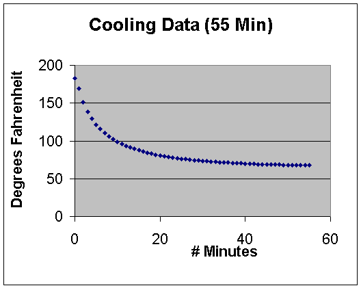
Excel provides a nice scatter plot of the data shown
below.
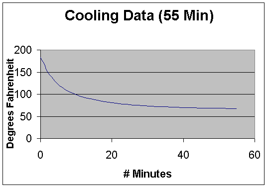
Another option Excel offers is to draw in a line
versus data points. Based on the graph
below, one might think that and accurate regression could be created, but this
is not the case…
When choosing a regression model it’s often helpful to consider the phenomenon you are observing. Will a liquid cooling fit a linear, quadratic, exponential, or some other model? This is a commonly know application of Newton’s Law of Cooling which is involves an exponential model, so let’s start there. Notice, the regression
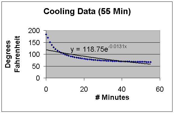
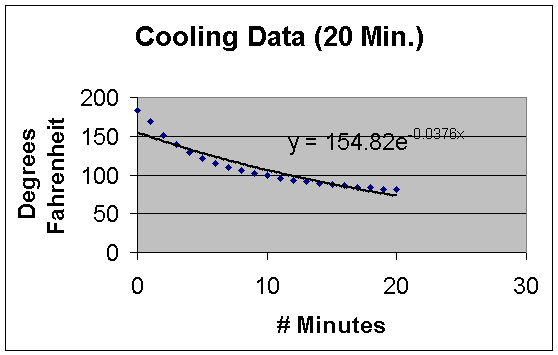
Notice, the regression doesn’t give such a good model. This is not a surprising result however, if you consider where the data points lie. Are the majority of the points in the curved part of the graph (left side), or where the graph flattens out? As you can see above, they are in the flatter part of the graph, which causes the regression model to be flatter that we wish. One way we could attempt to remedy this situation is to make a piecewise function where we approximate the left side using one function and the other part of the graph using a different function. Below, I used the first 20 minutes and found an exponential regression, the regression still fails to provide an accurate model.
Would Newton’s law do any better in this case? Newton’s Law of Cooling states that the rate of change of the temperature of an object is proportional to the difference between its own temperature and the ambient temperature (i.e. the temperature of its surroundings). It is represented by the equation:
T(t)
= Ta +(To + Ta)e-kt
T(t)
– Temperature at time t
Ta
– Ambient Temperature
To
– Original Temperature
k
– cooling constant
t
– time
Applying Newton’s Law of Cooling to our data, we obtain the equation
T(t)
= 67.53 + 115.67e0.0020847076t
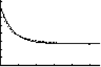
Using a TI-83 Plus Silver Edition, the following graph was produced. The x and y axes represent the same things as above. As you can see, this is a much better approximation.
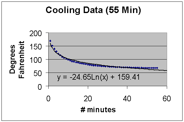
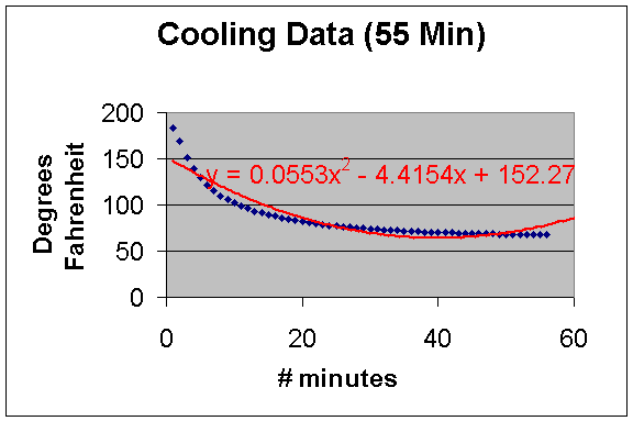
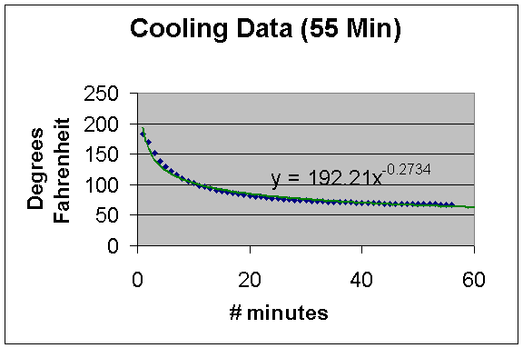
As a further exploration, I tried some different models to see which one actually Excel actually fit the data best with. The results are below. As you can see the power model and the logarithmic model give much better approximations.
Polynomial Model
Power
Model
Logarithmic Model
