An Attempt at Progress

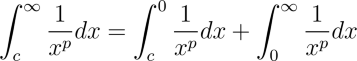
About a year before I met him, Ryan Fox wrote a most intriguing essay about improper integrals and their evaluation using technology (i.e. Maple). Knowing Ryan, I (moment of truth) Googled him and stumbled across his webpage. Having an interest in Maple, as evident in my 1st and 2nd essays, I began to expirement with his conjecture. Namely, he (along with some of his students, as you will learn through his essay) conjectured that

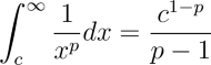
with certain restrictions on c and p. His desire was to demonstrate this using Maple, which is where I come in. One need only play with a few values of p before realizing that only three cases for p need to be considered. Namely, what happens for p > 1, p < 1, and p = 1? Similarly, three cases for c become necessary to check: c > 0, c < 0, and c = 0. Taking these together gives us 9 different ingtegrals to compute. Ryan and his students already computed some of them for several specific values of p and c. To do so in generality, one might be tempted to try all of them at once using the following method:

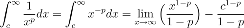
Then, you are left with 'simply' trying to compute a limit. One can tell, however, that this limit depends precisely on the cases outlined above. Let's see what Maple has to say about all of this. To check the different cases, we can use the assume command. This will tell Maple to assign properties to certain indeterminates. For example, we could say assume(t > 3); and Maple would do so. To undo this, we would need to execute t := 't'; and t would be stripped of all its previously imposed assumptions. So, let's lay out each of the 9 cases and see what Maple has to say about them. One note is in order - when Maple uses assumptions on an indeterminate, it denotes it with a tilda '~'. Thus, after executing assume(t > 3); typing t will return t~. Feel free to copy and paste the commands into Maple to see for yourself what is going on.

Case 1: p > 1, c > 0

> assume(c > 0, p > 1);
> simplify(int(1/x^p, x = c..infinity));

So far, so good. Let's quickly run through the other cases (unless, of course, something really weird happens, which is almost always). Remember, unless you execute restart; you need to run p := 'p'; and c := 'c'; before moving from case to case, though I won't show that here.

Case 2: p < 1, c > 0

> assume(c > 0, p < 1);
> simplify(int(1/x^p, x = c..infinity));

Well, that's a little weird, why did we get infinity? Take a look at the limit statement above. If p > 1 then 1 - p is negative, and so (mathematicians avert your eyes) we can think of having infinity on the denominator of the fraction (as the negative exponent moved it there from the numerator), but 1 on the top. 1 over very large numbers (approaching infinity) will get very small (approaching 0) so we just have Ryan's conjectured formula. If, however, p < 1 then 1 - p is positive and so we have infinity on the top (okay, large numbers approaching infinity) so we get something arbitrarily large over something constant minus something constant, which is arbitrarily large, so the limit is infinity. Now to case 3.

Case 3: p = 1, c > 0

> assume(c > 0, p = 1);
> simplify(int(1/x^p, x = c..infinity));

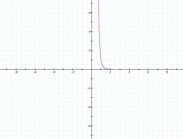
This one is a little stranger to think about. I think it's best to ignore the limit and look at the graph (thinking of the integral as the area between the graph and the x-axis).

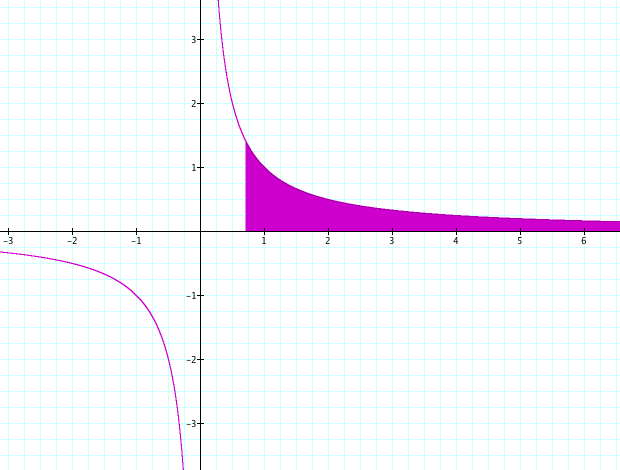
All Maple is saying is that there is an infinite amount of area below the purple line and above the x-axis, for any value of c > 0. This should come as no surprise to you Calculus buffs, but it is pretty cool anyway. Now for the other cases.

Case 4: p > 1, c = 0

> assume(c = 0, p > 1);
> simplify(int(1/x^p, x = c..infinity));

At first this looks like good news, because Maple keeps returning the formula or ∞. However, in case 4 c = 0, so why would Maple return c in the formula? This smells like a bug, and indeed it is. Let's give Maple a different set of commands and see what happens.

> assume(p > 1);
> simplify(int(1/x^p, x = 0..infinity));

That's a bit better. Maple is a powerful tool, but we need to double-check it when something smells fishy.

Case 5: p < 1, c = 0

> assume(c = 0, p < 1);
> simplify(int(1/x^p, x = c..infinity));

Again, this may be a bit weird to think about. Perhaps a proof by graph will convince you (it's a .mov file, so it'll play in Quicktime). As the value for p changes between -10 and 1, in each case the area in red is pretty obviously infinite. The spots where the graph is symmetric are those occuring when p is an integer, but since c = 0, we are only concerned with the area to the right of the y-axis (which is still infinite).

Case 6: p = 1, c = 0

> assume(c = 0, p = 1);
> simplify(int(1/x^p, x = c..infinity));

This is a special case that reverts to a familiar integration problem.

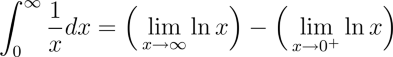
So we get a really big number subtracting a really small number and wham! we just keep heading to ∞.

Case 7: p > 1, c < 0

> assume(c < 0, p > 1);
> simplify(int(1/x^p, x = c..infinity));

Okay, this is really weird. Why in the world would we get that? Maybe more importantly, what is it that we got? The fact that we received ∞ times somthing is strange, but where did the exponential form come from? Let's take Maple's answer on faith for the moment, and play with it algebraically (at least the finite portion).

We know that

so, we could rearrange Maple's result to get

How should one think about such an expression? p > 1, so this seems to be giving us something like ∞ times some complex number. Fortunately, we can resolve it in a much simpler way. The graphs of the function for positive odd p all have something in common, they are all skew-symmetric (or odd, whichever terminology you prefer). Thus, they all lend themselves to the same basic solution, ∞. Check out case 9 for p = 1 and I'm confident you'll be able to fill in the details for other odd numbers. If p is even, then the graph of our function will be symmetric (or even), and so we definitely get ∞ (all the area is above the x-axis).

What if p is simply some non-integer positive real number? Then check out the graph:

The function has no real values for x < 0. Thus, it only makes sense to evaluate the integral from 0 onwards, which would seem to be ∞ like in case 4. Well, this still doesn't explain Maple's behavior, so let's continue to think about things. Maybe Maple broke the integral up into 2 pieces?

For the first piece, if evaluated with the assumptions that c < 0 and p > 1, Maple returns

and for the second piece

Now it's clear that Maple factored out ∞, which is somewhat unsettling. Let's focus on what Maple returned for the first part, the integral from c to 0. Applying our previous simplification, we get

Does this even make sense? Well no, notationally it presents some immediate problems, but can we see what Maple might be trying to say? The following (due to Brian Swanagan) is a possibility. Maybe Maple took the first integral (the one that gave us the exponential times infinity) and looked at it as a limit, and then tried to apply some algebra:

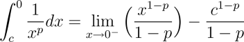
If so, then p > 1 would mean that the exponent 1 - p is negative. This would give us small numbers on the denominator and so large numbers as a whole. This limit seems to be -∞ with the value of (-1) to the -p multiplied as a scalar. Since the fraction after the limit (in the integral) doesn't have an x, it is finite and so doesn't change the limit. This is interesting, and may reflect what someone might be tempted to do. It is certainly interesting to think about more non-finite limits than just ∞ and -∞.

Case 8: p < 1, c < 0

> assume(c < 0, p < 1);
> simplify(int(1/x^p, x = c..infinity));

Here again, the function has no real values for x < 0 when p is a non-integer, so some of case 7 applies here as well.

Case 9: p = 1, c < 0

> assume(c < 0, p = 1);
> simplify(int(1/x^p, x = c..infinity));

Error, (in limit/mrv/limsimpl) too many levels of recursion

Now, this is just stupid. Depending on which version of Maple you are using, you may get a different result. Version 9.5 on the Mac gives me the above while on the PC, version 11 returns 'undefined.' I think both of these are results of bugs in the Maple code. Here's my thinking, let's look at the graph of the function, given these assumptions:

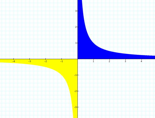
I've included the shading so we can remember that we're talking about area. Think of the yellow region as 'negative area' and the blue region as positive area (since that's what a definite integral would give us). Now, this graph is skew-symmetric, i.e. over the whole real range, the yellow or negative area exactly cancels the blue or positive area. Since we are taking an integral from x = c and c < 0 our integral is simply adding some of the yellow area (from x = c to x = 0) to all of the blue area. For example, if we had c = -2, the yellow area from x = -2 to x = 0 would cancel out the blue area from x = 0 to x = 2 and the integral would only return the area from x = 2 onward. The next picture will help explain:

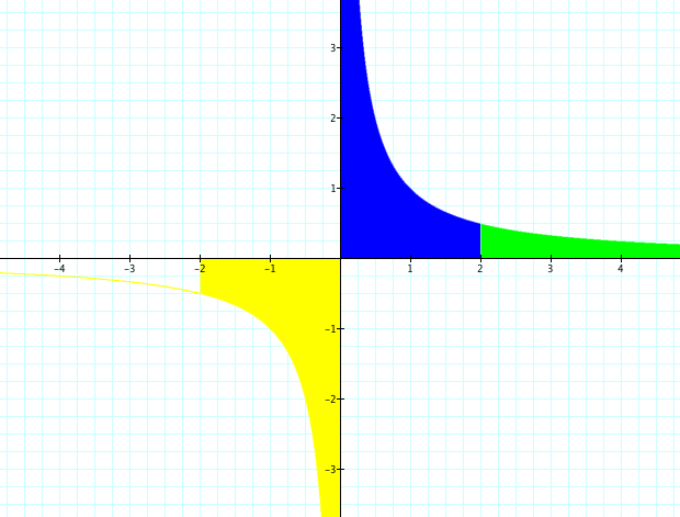
So, all the area from -∞ to -2 isn't counted (and so is not filled in) while the negative area from -2 to 0 (yellow) cancels the positive area from 0 to 2 (blue), leaving us with just the area from 2 to ∞ (green). Formally, we are saying that since

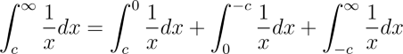
skew-symmetry gives us

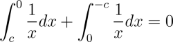
so all we're left with is the green area, which we can find by

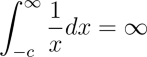
Now to recap the results of the 9 cases. When p ≤ 1, the integral evaluates as ∞, regardless of the value of c, which is also what we get for p > 1 and c = 0. When p > 1 and c > 0, Ryan's conjectured formula holds (or the formula conjectured by his student). When p > 1 and c < 0, weirdness happens, both mathematically and in Maple, where p an integer yields infinity but p a non-integer gives us trauma. Moral of the story: Maple is powerful, but it's not perfect (nor is any CAS), so do a reality check now and again.