Carisa
Lindsay
Assignment
10
Parametric
Equations Exploration
Suppose
we have the following equations:

For
simplicity, let’s investigate the graph for values of a = b and t-values between zero and 2p.
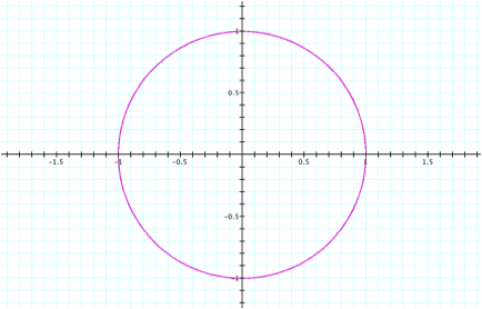
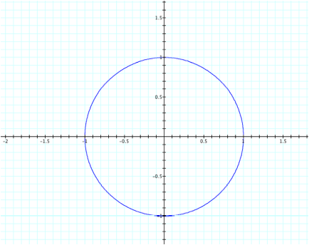
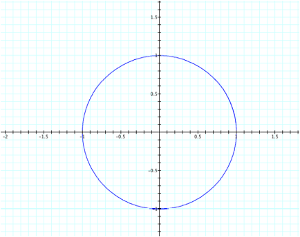
For
values of a = b greater than the absolute value of 1, we will get a circle of
radius 1 (not =0). For instance,
the following graph represents a = b = 3. Because we are dealing with a circle, it will not matter if
we use t-values larger than 2p
since the graph will continue along the circle.
Now
we can consider rational values of a
and b.
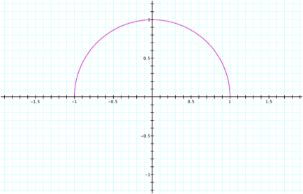
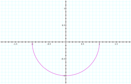
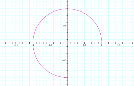
For
a = b =.5 and 0<t<2p,
we only see the top half of circle located in quadrants I and II.
However,
if we consider larger values of t, we will get slightly different results:
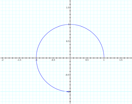
For
a = b =.5 and 0<t<3p
For
a = b =.5 and 0<t<4p

As
you can see, as we increase the range of t-values to include larger multiples
of Pi, we will again arrive at a circle.
If we try larger values of Pi, we will continue to get circles because
the graph will repeatedly create circles.
For
a = b =-.5 and 0<t<2p,
we see only the bottom half of the circle in quadrants III and IV.
Again,
if we increase the t-values to larger intervals of Pi, we will again arrive at
a circle.
a
= b=-.5 and 0<t<4p

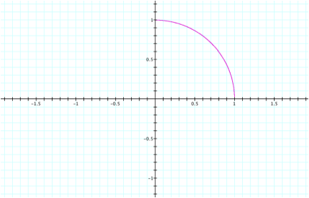
For
a = b =.25 and 0<t<2p,
we only see ¼ of the circle in quadrant 1
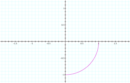
Likewise,
for a = b = -.25, we see ¼ of the circle in quadrant IV.
This
time, it will require us to use 0<t<8p
to get a full circle:
Quite
predictably, for a = b =.75 we see ¾ of circle in quadrants
I, II, and III.
Finally,
if a = b = -.75, our resulting circle resides in quadrants II, III, and
IV.

Lastly,
we can use 0<t<3p
to get a full circle for the above values of a = b = .75
or -.75:
For
a ¹
b, the graphs become quite
interesting. However, the t-values
seemingly do not affect how many “loops” each of the following graphs. For
simplicity’s sake, we will maintain the values of t to remain between 0 and
2pi.
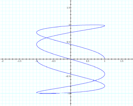
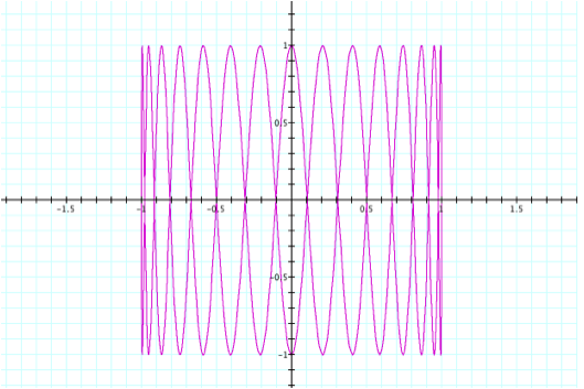
For
a = 1 and b any natural number, the number of “loops” corresponds to the
value of b. For instance, in the following graph, for a = 1 and b = 4, there are 4 “loops”.
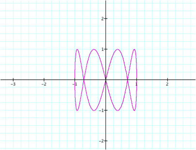
As
b increases, so do the number of
“loops”.
Suppose
we consider large values of b. For
instance, let a= 1 and b = 15.
According to the pattern seen thus far, we should see 15 “loops”.
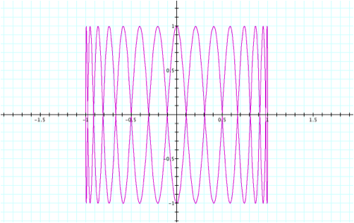
As
predicted, we see 15 “loops”. What
about a = 1 and b = 50?
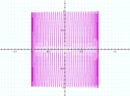
Please
note that for all of these values, the graph oscillates between -1<x<1
and -1<y<1.
However,
if we explore negative values of b,
we see the same picture.
What
about rational values of b? For values between 0 and 1, the graph
appears to behave much like a slinky.
Again, we have oscillatory motion for -1<y<1 and -1<x<1. As b approaches 1, the graph appears
more like a circle and will eventually be a circle for b = 1.
Suppose
we change the values of a
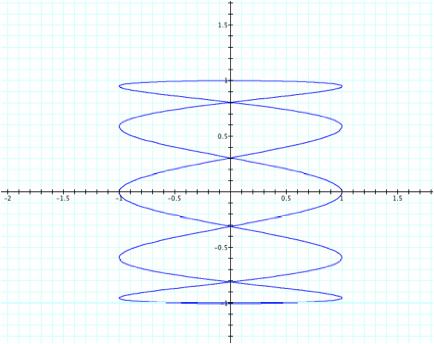
and keep b = 1. For a values between 0 and 5, the
graph follows a similar oscillatory pattern except in a vertical fashion. These graphs also have a domain of
-1<x<1 and a range of -1<y<1. Obviously, the values of a and b control which direction the graph oscillates. Unlike the values of b, the number of
waves also corresponds to the value of a for odd values.
For even values of a, we see
the period corresponds to half the value of a.
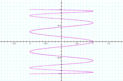
For
instance, suppose a = 5 and b = 1. We can predict a graph with vertical oscillations and 5
“loops”.
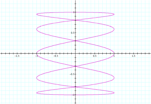
Now
suppose a = 10 and b =1. We can predict another graph with vertical oscillations and 5
periods.
To
see other values of a, Click here for animation. This animation has 0<a<6, b=1, and
0<t<2Pi.
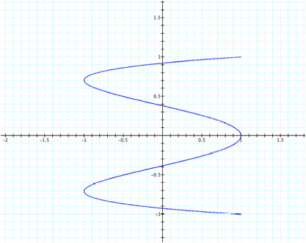
Perhaps
some of the more interesting observations are when a is
a whole number, the graph is continuous.
When a=1, we again see a circle; if a =2, we see a sideways parabola; if
a=3, we see a vertical “spring” with 3 “loops”; if a=4, it resembles a=2 with
an extra curve; and a=5 has 5 “loops”.
It appears that for odd-values of a, we will see a figure that is “closed”
meaning that it will continue along that path without having to move
backwards. For instance, an object
can continue to travel along a circular path forever.
However,
for even values of a, we will result in a graph that is not “closed”:
When
we use negative values of a, we get
similar results as when b was
negative. In fact, the graph is
identical to the resultant graph from positive values of a. Essentially, we are
only interested in the absolute value of a
since the graph is the same for negative values of a.
For
rational values of a, we see similar
oscillatory motions except that the movements are horizontal. Furthermore, all non-whole values of a
will result in a graph that is not “closed”: