Fibonacci Sequences
By Pei-Chun Shih
In
the year 1202, the Italian mathematician Leonardo de Pisa, best known as
Fibonacci, presented his famous findings about how fast rabbits could breed in
ideal circumstances.
Here
are the assumptions:
1. Suppose a newly-born pair of rabbits, one male, one
female, are
allowed to breed in a controlled environment.
2. Rabbits are able to mate at the age of one month.
3. At the end of its second month a female can produce
another pair of
rabbits.
4. The rabbits never die and the female always produces one new pair
(one male, one female) every month from the second month on.
How
many pairs will there be in one year?
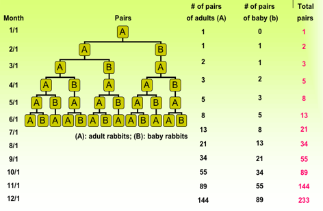
There
will be 233 pairs of rabbits during the twelfth month.
The
rabbits’ problem generated the following sequence of numbers: 1, 1, 2, 3, 5, 8,
13, 21, 34, 55, 89, 144, 233, …, which is known today as the Fibonacci
Numbers and the sequence is called
the Fibonacci Sequence. Every
numbers in the Fibonacci sequence (after the first two) is the sum of the
two preceding numbers. Therefore, the
Fibonacci numbers can be defined as the linear recurrence equation: Fn = Fn-1 + Fn-2
with F0 = 0 and F1 = F2 = 1.
Hence,
F3 = F2 + F1 = 1 + 1 = 2
F4 = F3 + F2 = 2 + 1 = 3
……
F13 = F12 + F11 = 144 + 89 = 233, and so on.
After
understanding the origin of the Fibonacci numbers and sequence, I am going to
use the spreadsheet to do some explorations.
First,
I generate a Fibonacci sequence in the second column of the spreadsheet using
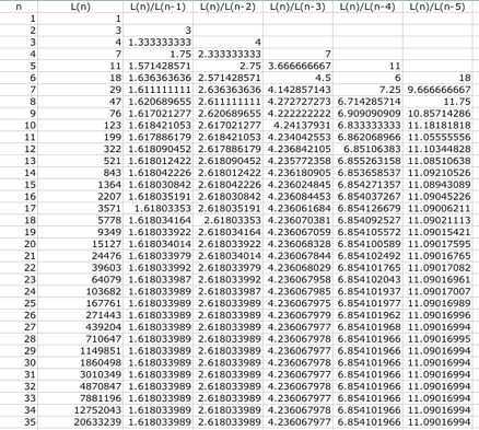
F(0) = 1 and F(1) = 1. Second, in the third column I construct the ratio of
each pair of adjacent terms in the Fibonacci sequence, that is Fn/Fn-1.
In the fourth column, I construct the ratio of every second term in the
Fibonacci sequence. Likewise, the fifth column is the ratio of every third term
in the Fibonacci sequence, and the sixth column is the ratio of every fourth
term in the Fibonacci sequence, and so forth.
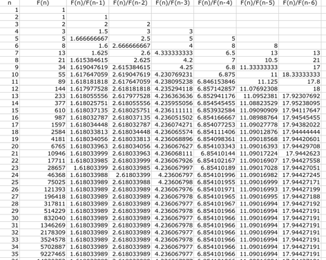
As
we can see from the third column, as the numbers get larger, the ratio seems to
approach a specific number. What is this specific number that the ratios are
approaching?
Let’s
sketch a diagram to help us visualized the pattern. Let n be the x-coordinate
and (Fn / Fn-1) be the y-coordinate.
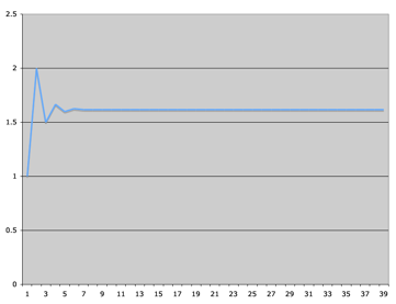
The
diagram above also shows that the ratio of two neighboring Fibonacci numbers
soon settled down to a particular value near 1.61803 as n increases. This
specific number, 1.618033989, is known as the Golden Ratio.
The
numbers in the fourth column, which are the ratios of every second term, also
approach to a specific number as n getting large. This specific number is the
second power of the golden ratio, that is (1.618033989)2 =
2.618033989. Similarly, the numbers of the fifth column come close to the third
power and the sixth column to the fourth power of the golden ratio as n
increases.
Another
interesting discovery can be found from the spreadsheet above that the first
two cells of each column also form the Fibonacci numbers.
Although
the Fibonacci numbers had existed since the year 1202, they didn’t get too much
attention until a French mathematician, Edouard Lucas (1842-1891), studied them
in the second half of the nineteenth century. He was curious about the start of
the Fibonacci sequence and wondering what would happen if the sequence had
begun with 1 and 3. So he started his number with 1 and 3, rather than 1 and 1
and followed the same additive rule as the Fibonacci numbers. He found that the
Lucas numbers, which are 1, 3, 4, 7, 11, 18, 29, 47, 76, 123, …, interconnect
with the Fibonacci numbers. Here I am going to use the spreadsheet to explore
their relationship.
In
the spreadsheet above, I generated the Lucas numbers using the same technique I
did in generating the Fibonacci numbers earlier. From the third column above,
it also shows that the ratio of two neighboring Lucas numbers soon settled down
to the golden ratio, 1.618033989, as n increases.
Like
the ratios of the Fibonacci numbers, the Lucas numbers in the fourth column,
which are the ratios of every second term, also approach to the second power of
the golden ratio, that is (1.618033989)2 = 2.618033989. Similarly,
the numbers of the fifth column come close to the third power and the sixth
column to the fourth power of the golden ratio as n increases. Likewise, the
first cell of each column also forms the Lucas numbers.
Now
we know that both the Fibonacci and the Lucas sequences approach the golden
ratio. Do they have direct connection with each other? Let’s use the
spreadsheet to try to relate these two sequences directly.
After
several attempts, I realized there is a direct connection between these two
sequences. The nth Lucas number (n ³ 0) is equal to the sum of the (n-1)st
Fibonacci number and the (n+1)st Fibonacci number. That is: Ln = Fn-1 + Fn+1.
In the diagram below, you can observe
this relationship from the first four columns where the sequences placed next
to each other.
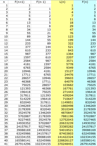
When
is a Fibonacci number equal to a Lucas number?
From
the spreadsheet above, it seems that they only equal at the very first
beginning, that is F1 = L1 = 1, F2 = L1
=1, and F4 = L2 = 3. They have never got any other chance
to be equal as n increases.
I
will close this write-up with the following question: can we use GSP to
generate the Fibonacci sequence? The answer is yes, but how?
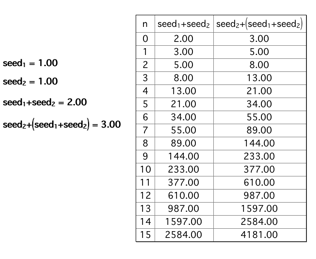
First,
we have to define the starting value of the sequence and the difference. GSP
uses “seed” as the command to generate a sequence. In order to differentiate
the sequence, GSP uses square brackets [] to indicate the number within will be
a subscript. Thus, “seed [1]” will define the first term of the arithmetic
sequence. But where should we place the command?
Choose
Calculate under the menu of
Measurement. Select Value then New Parameter. In the box for Name, type “seed [1]”. In the box for Value, type 1. Also define seed [2] = 1 in the same way.
These two steps define the first and the second terms of the Fibonacci numbers.
Use Calculate to calculate
“seed1 + seed2” and “seed2 + (seed1
+ seed2)” which is the third and the fourth terms respectively.
Second,
we need to know how the Transform menu’s Iterate
command functions. According to the help menu of the GSP, Iterate command enables you visualize the orbit of one or
more objects over some number of repetitions of a construction. Therefore, by
selecting seed1 and seed2, then choose Iterate from the Transform menu and do things like the diagram below, we can
generate the Fibonacci sequence we want.
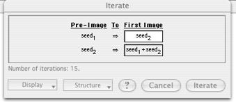
The
idea here is to iterate with seed1 = 1 mapped to seed2 =1
and seed2 =1 mapped to (seed1 + seed2) = 2.
You can choose the number of iterations at the Display dialog box.
Voila!
Here is the Fibonacci numbers generating by GSP.
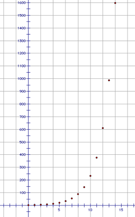
The
last, I plot the Fibonacci numbers to help visualize the dramatic change of
them. The plot below shows how fast and steeply the values grow.