We are going to study some equations written in polar form. Remember that the coordinate plane is the same and the points have not moved. We just write their addresses differently. Why would we ever want to do that? Some equations are simpler written in polar format than in rectangular format.

If you would like some polar graph paper to make it easier to approximate your angles, click here to download a free printable sheet.

Let's start by looking at a few graphs to see what to expect when we try our first one.

Check this one out.

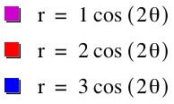To understand this fully, we will have to look at a few specific ordered pairs, but if we compare these three equations, we can tell that changing the coefficient of the cosine changes nothing but the amplitude. So for the rest of our graphs, we will leave this value set at 1 and consider changing the coefficient of theta.

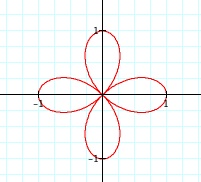
So, we will start with a graph of and think about specific points that create this graph.

Let's make a table of values to get us started.

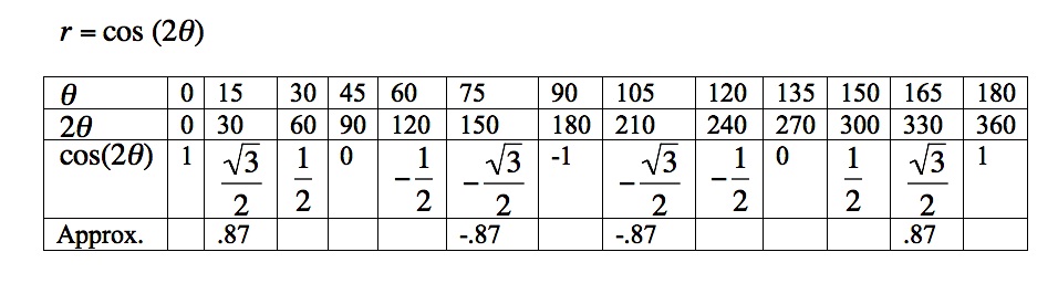
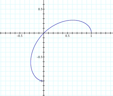
If we compare the table of values to the portion of the graph at the left, we notice that as theta goes from 0 to 45, 2 theta goes from 0 to 90. If we think about the cosine function, we know that between 0 and 90 the cosine function decreases from 1 to zero. So, if we look at the portion of this graph in the first quadrant of the rectangular coordinate plane, we see the distance from the each point to the pole decreasing from 1 to 0 as the angle moves from 0 to 45 degrees.

Then as theta moves from 45 to 90, 2 theta moves from 90 to 180. In this interval, the cosine function decreases from 0 to -1, so we have to think about graphing negative values. Remember that to do this, we move through the angle and move the specified number of units in the opposite direction. So, instead of being in the first quadrant, the points are in the third quadrant, moving from zero to -1.

Look at the rest of the values in the table, theta moving from 90 to 180 as 2 times theta moves from 180 to 360. Try graphing this set of points yourself before you scroll down to look at the next graph. Where do you think this curve is going next?

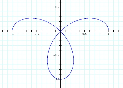
As theta moves from 90 to 135, 2 times theta moves from 180 to 270, and the cosine function moves from -1 back to 0. So as we graph these points we rotate to the second quadrant, but move on the ray in the "negative" direction so our points are in the fourth quadrant - moving from -1 back to zero. Then as theta moves from 135 to 180, twice theta moves from 270 to 360 and the cosine function moves from 0 to 1. Those are positive values so they graph in the second quadrant. Remember the points we are graphing are these distances from the pole. The numbers that you see on the graph at the right are rectangular coordinates - which we are not using right now.

This graph doesn't appear to be finished yet. So, let's look at what the cosine curve is doing to complete this graph. The cosine curve is graphed below to help us think.

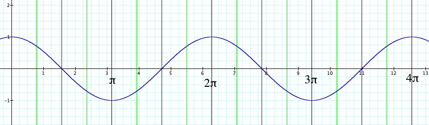
Look at the cosine function and think of the next set of values. As theta moves from 180 to 225, twice theta moves from 360 to 450. Find this interval on the graph above and see what the cosine is doing there.

We should be moving from 1 to zero in this interval.  Draw your own graph through this interval. 

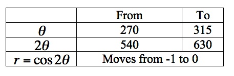
Next, as theta moves from 225 to 270, twice theta moves from 450 to 540.  Look at the graph of the cosine curve above, think where the graph should go next and continue your graph.  Then scroll down to check.

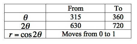
We are almost done.  Look at the following two intervals and complete your graph.

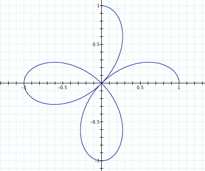
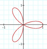
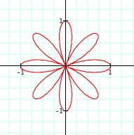
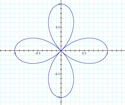	So, we have completed the graph of the four petal rose at the left.  Now that we are more familiar with graphing using polar coordinates we can look at some completed graphs below.

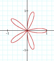 What do you notice about the number of "petals" related to the equations?