An Introduction to Parametric Equations
by
Jackie Ruff
After
studying equations of lines, linear relationships and their slope in
the traditional way, let's look at them in a different way. We
can write an equation for a line by defining the coordinates of our
solutions with two continuous functions in terms of another variable,
say t.
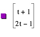
Suppose we want to find an equation for a line segment that goes through (4, 5) and has a slope of 2. One way would be to write the equation the way that we normally do. Using the point-slope form to write the equation we have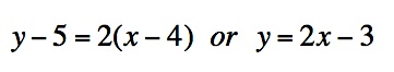 . So, we could write, x = t + 1 (an arbitrary relationship for the sake of example) and
substituting this expression for x and solving for y, we have y = 2t - 1.
Take a look at the graph. Obviously it is graphing our line only for certain values of t, from -1 to 1.
So, we have to think about setting the range of the parameter to show the portion of the graph which interests us for a particular situation.
Parametric equations provide a way to consider a situation using more than the two variables - which sometimes makes a problem easier to analyze.
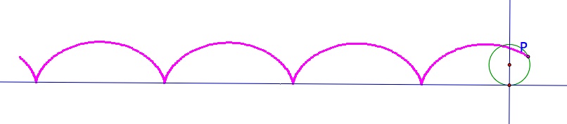
Let's consider finding the locus of a point as it rotates around a circle that is rolling on a flat surface. So, we will look at the picture below and think of a way to describe the point P. Point P was initially at (0, 0) on a radius perpendicular to the horizontal line .
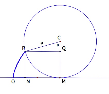 The radius of circle C is a.
Point P is an arbitrary point on the circle. CM is now
perpendicular to the line the circle is rolling on. The circle
has rolled on the flat surface and point P has rotated around - its
path has been traced. So OM, the distance that the circle has
rolled over, is equal to arc MP. That means that segment CP has
rotated through angle theta. PQ has been drawn parallel to line
NM and PN has been drawn parallel to CM. Using right triangle CQP, we
have
The radius of circle C is a.
Point P is an arbitrary point on the circle. CM is now
perpendicular to the line the circle is rolling on. The circle
has rolled on the flat surface and point P has rotated around - its
path has been traced. So OM, the distance that the circle has
rolled over, is equal to arc MP. That means that segment CP has
rotated through angle theta. PQ has been drawn parallel to line
NM and PN has been drawn parallel to CM. Using right triangle CQP, we
have 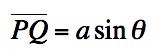 . We also have that
 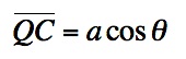 .
To find coordinates for point P, we need an expression for the distance
from (0,0) and N and for the length of segment NP. NP = MQ which
is the same as (a - CQ). So,
.
To find coordinates for point P, we need an expression for the distance
from (0,0) and N and for the length of segment NP. NP = MQ which
is the same as (a - CQ). So, 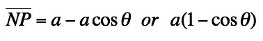 . Now, ON equals OM - NM. NM = PQ. Remember that OM is the same as arc PM.
  .
.
So,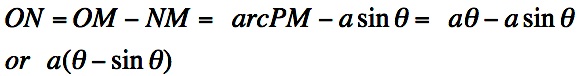 .
.
So, the coordinates for point P are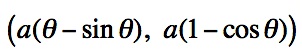 in terms of a, the radius of the circle.*
We can graph the parametric equations,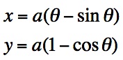 to find the locus of point P as the circle rolls.
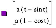
 . Here, the value of a, the radius of the circle, is 1.
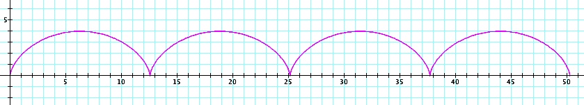
Changing the radius to 2, we have this graph: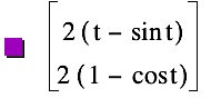
We can also look at a geometric construction of this locus. See the picture below, or click here to view the animation in a Geometer's Sketchpad file.
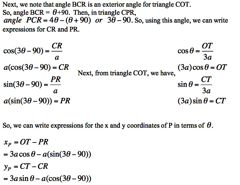
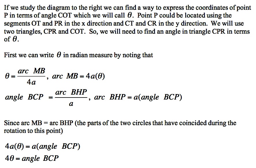
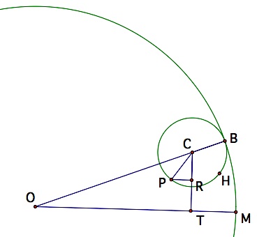
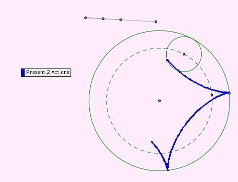
Let's consider a similar problem where a circle rotates around the inside of another circle while we trace the locus of a point on the smaller circle. In the circle to the right, OB = 4a. The radius of circle C is a. Point P was initially at the location of point M. It has rotated to its current position.
If we graph this locus of points, we have the following.
Suppose we want to find an equation for a line segment that goes through (4, 5) and has a slope of 2. One way would be to write the equation the way that we normally do. Using the point-slope form to write the equation we have
. So, we could write, x = t + 1 (an arbitrary relationship for the sake of example) andsubstituting this expression for x and solving for y, we have y = 2t - 1.
Take a look at the graph. Obviously it is graphing our line only for certain values of t, from -1 to 1.
 | 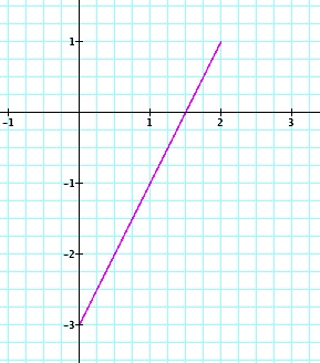 |
So, we have to think about setting the range of the parameter to show the portion of the graph which interests us for a particular situation.
Parametric equations provide a way to consider a situation using more than the two variables - which sometimes makes a problem easier to analyze.
Let's consider finding the locus of a point as it rotates around a circle that is rolling on a flat surface. So, we will look at the picture below and think of a way to describe the point P. Point P was initially at (0, 0) on a radius perpendicular to the horizontal line .
The radius of circle C is a.
Point P is an arbitrary point on the circle. CM is now
perpendicular to the line the circle is rolling on. The circle
has rolled on the flat surface and point P has rotated around - its
path has been traced. So OM, the distance that the circle has
rolled over, is equal to arc MP. That means that segment CP has
rotated through angle theta. PQ has been drawn parallel to line
NM and PN has been drawn parallel to CM. Using right triangle CQP, we
have . We also have that .
To find coordinates for point P, we need an expression for the distance
from (0,0) and N and for the length of segment NP. NP = MQ which
is the same as (a - CQ). So, . Now, ON equals OM - NM. NM = PQ. Remember that OM is the same as arc PM. . So,
. So, the coordinates for point P are
in terms of a, the radius of the circle.*We can graph the parametric equations,
to find the locus of point P as the circle rolls.. Here, the value of a, the radius of the circle, is 1.Changing the radius to 2, we have this graph:
We can also look at a geometric construction of this locus. See the picture below, or click here to view the animation in a Geometer's Sketchpad file.
Let's consider a similar problem where a circle rotates around the inside of another circle while we trace the locus of a point on the smaller circle. In the circle to the right, OB = 4a. The radius of circle C is a. Point P was initially at the location of point M. It has rotated to its current position.
 |  |
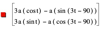
If we graph this locus of points, we have the following.
 |  |
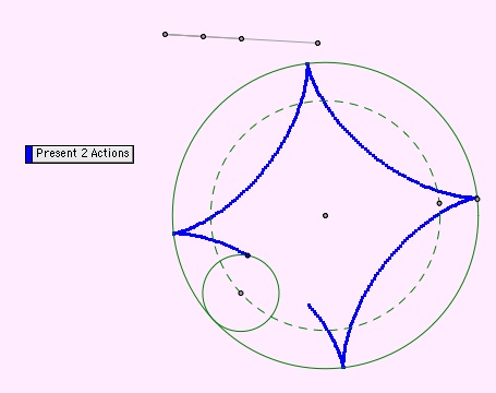
We can construct this same locus of points by allowing a circle to roll around the inside of a larger circle as we trace an arbitrary point on the smaller circle.
Here are a few action shots.
Then, you can open this file and animate it yourself.