
Assignment 11: Problem 2
Jason P. Pickhardt
Problem:
Investigate varying a and k:
1. ![]()
2. ![]()
Exploration:
This exploration was done using Graphing Calculator software. For ease of exploration we will start with a=1 and vary k for the first two equations to investigate. Note that the graphs in purple represent equation 1 and the red graphs represent equation 2. Plugging in for a=1 our equations become:
1. ![]()
2. ![]()
Let’s try the following set of values for k to see if we can come up with some generalizations about the results of varying k in these equations:
k = {1,2,3,4}
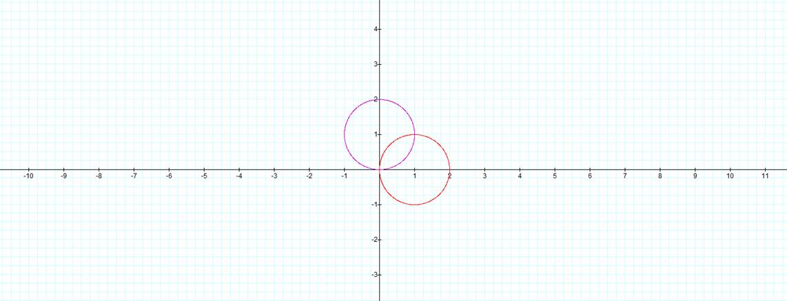
When k=1 our equations become:
1. ![]()
2. ![]()
The following figure contains the graphs of these equations
over the interval![]() :
:
It is important to know that:
![]()
![]()
![]()
Knowing this, it is
possible to calculate some values of r
and coordinates (x, y) in order
compare our results to the graphs of the equations. Let’s try values of ![]() over the interval of
over the interval of![]() for equations 1 and 2.
for equations 1 and 2.
|
|
r |
(x, y) |
|
0 |
0 |
(0,0) |
|
|
|
(1,1) |
|
|
2 |
(0,2) |
|
|
|
(-1,1) |
|
|
0 |
(0,0) |
|
|
|
(1,1) |
|
|
2 |
(0,2) |
|
|
|
(-1,1) |
|
|
0 |
(0,0) |
Solutions for equation 1.
|
|
r |
(x, y) |
|
0 |
2 |
(2,0) |
|
|
|
(1,1) |
|
|
0 |
(0,0) |
|
|
|
(1,1) |
|
|
2 |
(2,0) |
|
|
|
(1,1) |
|
|
0 |
(0,0) |
|
|
|
(1,1) |
|
|
2 |
(2,0) |
Solutions for equation 2.
In order to find the coordinates for each point we need to substitute the radius and degree to the equations given for x and y. Notice that indeed the solutions shown in the previous tables describe the graphs for equations 1 and 2. Now we can continue in the same manor for the rest of the values of k we desired to explore. The following are the graphs of equations 1 and 2 for k=2 which are written:
1. ![]()
2. ![]()
As we did for our first case, let’s try to figure out the
radius and coordinates for angles of![]() on the interval
on the interval![]() .
.
|
|
r |
(x, y) |
|
0 |
0 |
(0,0) |
|
|
2 |
( |
|
|
0 |
(0,0) |
|
|
-2 |
( |
|
|
0 |
(0,0) |
|
|
2 |
( |
|
|
0 |
(0,0) |
|
|
-2 |
( |
|
|
0 |
(0,0) |
Solutions for equation 1.
|
|
r |
(x, y) |
|
0 |
2 |
(2,0) |
|
|
0 |
(0,0) |
|
|
-2 |
(0,-2) |
|
|
0 |
(0,0) |
|
|
2 |
(-2,0) |
|
|
0 |
(0,0) |
|
|
-2 |
(0,2) |
|
|
0 |
(0,0) |
|
|
2 |
(2,0) |
Solutions for equation 2.
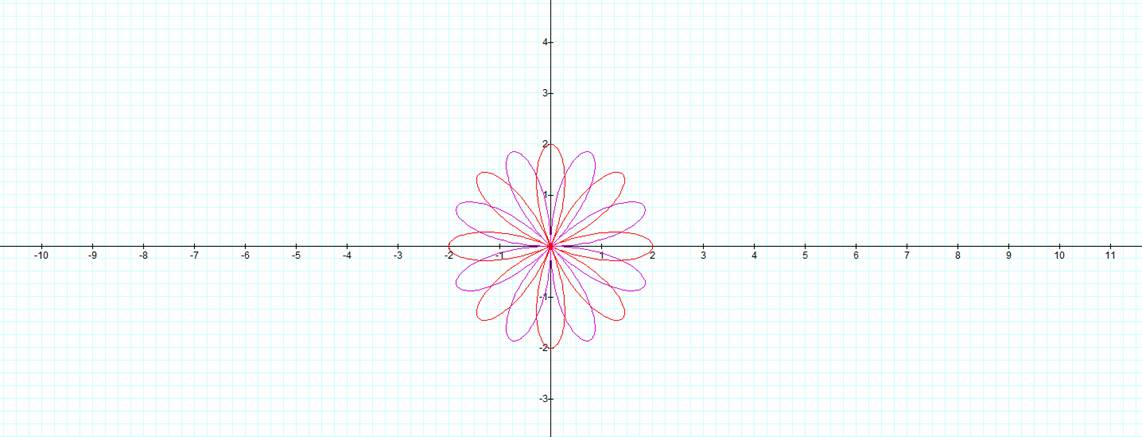
When analyzing the coordinates over the given interval we can see that the graphs of the equations are creating the “pedals” in a clockwise manor. The curvature in between each of the points is caused by the fact that we are using sine and cosine functions to create these coordinates. Let’s proceed as in the previous cases for k=3 and k=4.
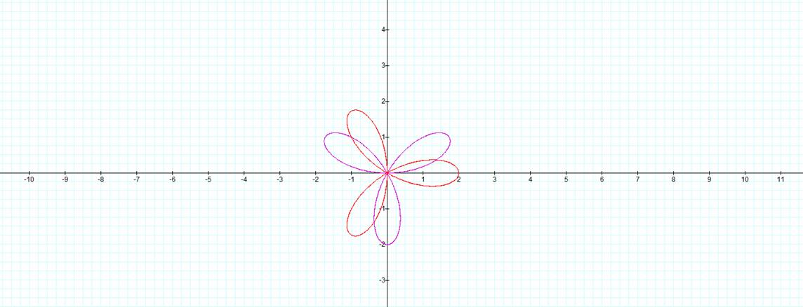
k = 3
1. ![]()
2. ![]()
|
|
r |
(x, y) |
|
0 |
0 |
(0,0) |
|
|
|
(1,1) |
|
|
-2 |
(0,-2) |
|
|
|
(-1,1) |
|
|
0 |
(0,0) |
|
|
|
(1,1) |
|
|
2 |
(0,-2) |
|
|
|
(-1,1) |
|
|
0 |
(0,0) |
Solutions for equation 1.
|
|
r |
(x, y) |
|
0 |
2 |
(2,0) |
|
|
|
(-1,-1) |
|
|
0 |
(0,0) |
|
|
|
(-1,1) |
|
|
-2 |
(2,0) |
|
|
|
(-1,-1) |
|
|
0 |
(0,0) |
|
|
|
(-1,1) |
|
|
2 |
(2,0) |
Solutions for equation 2.
We can see from the previous tables that we are missing some values for our graphs. However, we can check the coordinates that we do have and see that they do lie on the graphs produced in Graphing Calculator.
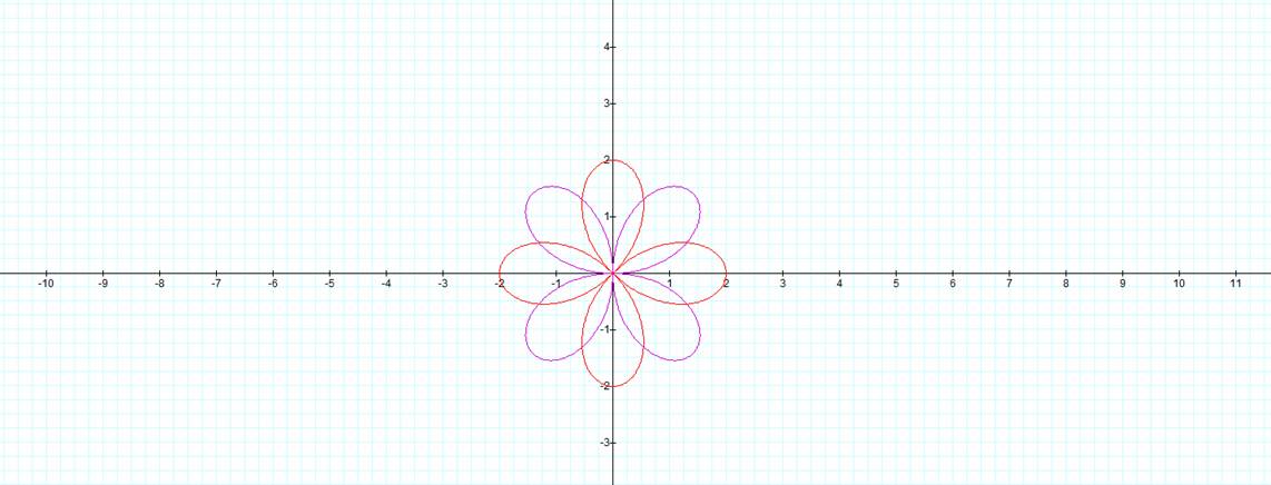
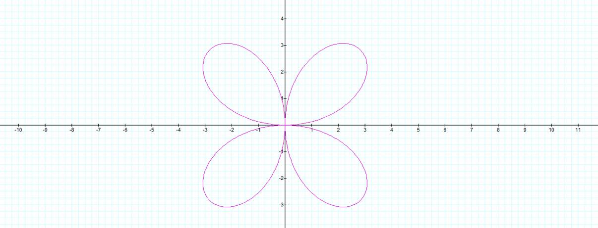
k = 4
1. ![]()
2. ![]()
|
|
r |
(x, y) |
|
0 |
0 |
(0,0) |
|
|
0 |
(0,0) |
|
|
0 |
(0,0) |
|
|
0 |
(0,0) |
|
|
0 |
(0,0) |
|
|
0 |
(0,0) |
|
|
0 |
(0,0) |
|
|
0 |
(0,0) |
|
|
0 |
(0,0) |
Solutions for equation 1.
|
|
r |
(x, y) |
|
0 |
2 |
(2,0) |
|
|
-2 |
( |
|
|
2 |
(0,2) |
|
|
-2 |
( |
|
|
2 |
(-2,0) |
|
|
-2 |
( |
|
|
2 |
(0,-2) |
|
|
-2 |
( |
|
|
2 |
(2,0) |
Solutions for equation 2.
In this case the table of coordinates does not help us confirm our graphs. However it should be rather intuitive given the amount of pedals in these graphs that they go through the points (0,0) for equation 1 and those points given for equation 2 multiple times. We have not yet explored the possibility of varying the value of a in our equation. If we look at the equation we realize that this will not yield a particularly interesting result. Changing the value of a will simply stretch our graph. Let’s take the coordinates for equation 1 when k=2 and a=2. The graph and resulting table of coordinates would look as such.
1. ![]()
|
|
r |
(x, y) |
|
0 |
0 |
(0,0) |
|
|
4 |
(2 |
|
|
0 |
(0,0) |
|
|
-4 |
( |
|
|
0 |
(0,0) |
|
|
4 |
( |
|
|
0 |
(0,0) |
|
|
-4 |
( |
|
|
0 |
(0,0) |
Solutions for equation 1.
We can see that by using a value of k=2 that we doubled the radius at each point as well as the coordinates. When we have k=3 these values will triple, k=4 they will quadruple and so on in the same manor. If it suits the reader these constructions can easily be made and checked in Graphing Calculator.
Conclusion:
We saw by participating in this exploration how polar and Cartesian coordinates interact to give us some interesting figures. The figures we created had pedals whose numbers were defined by the parity of k. That is, when k is even we have 2k amount of pedals and when k is odd we have k number of pedals. Also, we realized that varying a stretches or shrinks our graphs by some multiple or fraction of 2. There seems to be a multitude of possibilities when exploring further with these types of polar equations but this will serve as the end of our exploration here.