
Assignment 2: Problem 4
Jason P. Pickhardt
Problem:
Graph the parabola:
![]()
i. Overlay a new graph replacing each x by (x - 4).
ii. Change the equation to move the vertex of the graph into the second
quadrant.
iii. Change the equation to produce a graph concave down that shares the same
vertex.
iv. Generalize . . .
Note:
Using a program such as Graphing Calculator it would be easy to graph the given quadratic equation. Also, we could do some simple algebraic manipulation to replace x by (x-4) and overlay the necessary graph. However, when we get to the latter parts of the problem it is necessary to know some things about transforming quadratic equations. Thus it seems necessary to explore some quadratic functions to generalize the transformations before completing parts i-iii. The following is a summary of the exploration I completed in order to answer the problem.
Exploration:
When working with functions it is sometimes useful to begin with a parent function. In the case of our given problem, the parent function is a simple parabola described by the following:
![]()
Knowing this, we can begin to explore how to transform the
parent function in order to find our desired quadratic equation. We can also
begin to form some ideas for generalizing the transformations of a quadratic
equation. Let’s being with increasing and decreasing the coefficient of the
parent function![]() , for instance consider the following two equations graphed
using the Graphing Calculator software along with the parent function.
, for instance consider the following two equations graphed
using the Graphing Calculator software along with the parent function.
![]()
![]()
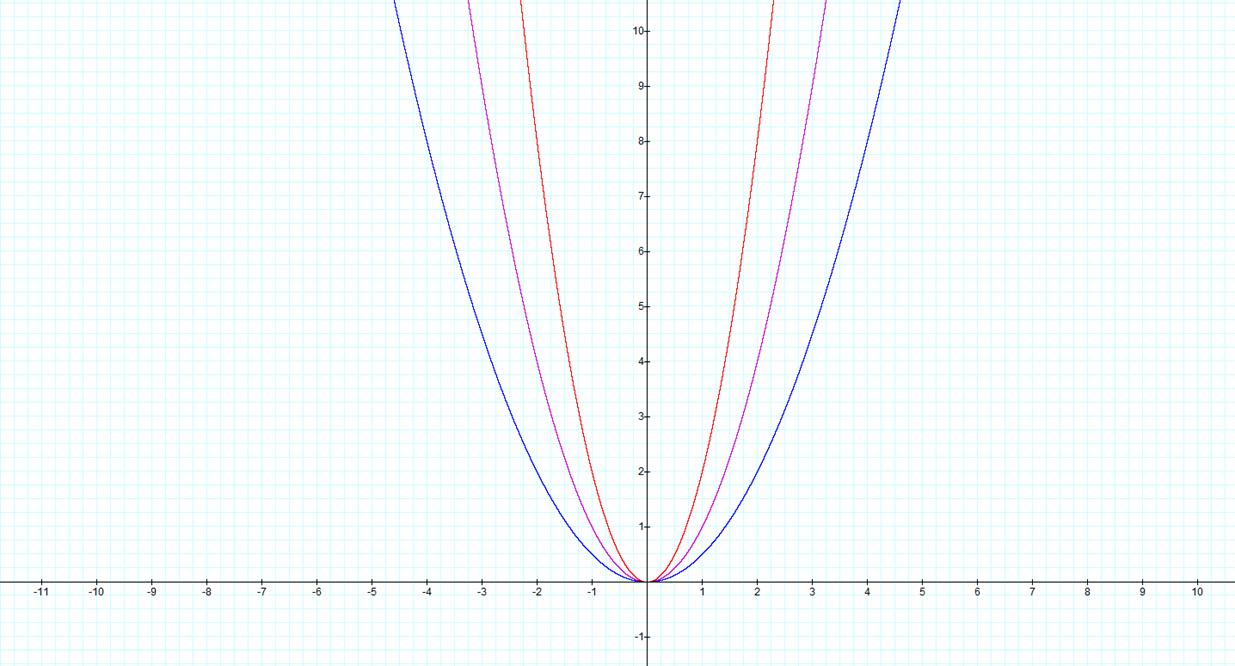
Figure1- For
further reference the parent function ![]() will be graphed in purple while
new equations will be highlighted with respect to their graphed color as shown
above.
will be graphed in purple while
new equations will be highlighted with respect to their graphed color as shown
above.
We can see in figure 1 that increasing the coefficient of the parent function shrinks the graph of the function while decreasing the coefficient stretches the graph. It is also necessary to note that each of the three graphs is figure 1 share the same overall shape as well as the same vertex of (0,0). While this information is interesting, it is necessary to continue our exploration. Now we can add different values of x to the parent function to see what type of transformation results. The following are four different types of equations we could write and their corresponding graphs:
![]()
![]()
![]()
![]()
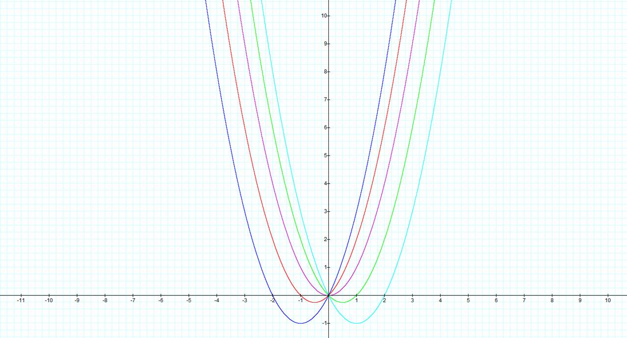
Figure 2-
Adding values of x to the parent
function
It is considerably harder to evaluate what type of
transformation is happening here. However, one thing that we can conclude right
away is that there is no shrinking or stretching happening when we add a value
of x. Also, we can see that when we
add a positive value of b the graph
shifts to the left and similarly adding a negative value of b shifts our graph to the right. It
remains to discover what is happening to the vertex of the graph since none of
these equations shares the same vertex. After going over many more examples it
is possible to find a generalization for how the vertex is transformed. We must
consider the general equation ![]() when devising rules for
this transformation, which are as follows:
when devising rules for
this transformation, which are as follows:
a>0 & a<0, b>0 vertex moves by 
a>0 & a<0, b<0 vertex moves by 
The last item we need to explore is adding a constant to the parent function. We can add a value of 1 or -1 to the parent function and get the following:
![]()
![]()
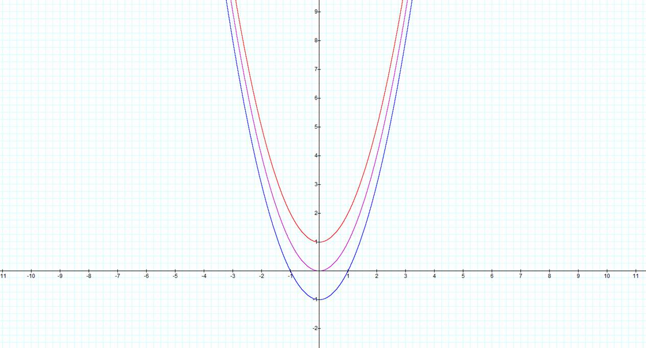
Figure 3-
Adding a constant to the parent function
It is fairly easy to see from figure 3 that adding a constant
shifts the graph vertically by the value of the constant. It remains now to use
this knowledge to answer the questions at hand. Thus we must first graph the
original equation of![]() . For the sake of brevity we can also complete the case where
x is replaced by (x-4) in the same graph. The results are as follows:
. For the sake of brevity we can also complete the case where
x is replaced by (x-4) in the same graph. The results are as follows:
![]()
![]()
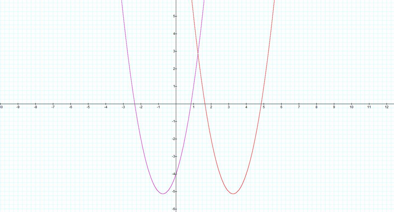
Figure 4-
Graph of original equation and part (i)
We can check our original findings against what we have graphed here. If we were to simplify the case were x is (x-4) we would come up with:
![]()
We know instantly that the graph should shrink by a factor of 2 given the coefficient in front of the squared term. Also, we know the vertex will shift at the very least +16 units in the vertical direction. It now remains to see what effect the x term has on the vertex. From the formulas we came up with the middle term would shift the vertex by (3.25, -21.125). Adding the +16 units in the y-direction we end up with a vertex of (3.25, -5.125) Using the Graphing Calculator software we can check and conclude that indeed this is the correct vertex. Thus, we have shown that our findings from earlier work. Using the principles from the exploration we can find equations to satisfy part ii and iii of the problem. They are written and graphed as follows:
ii) ![]()
iii) ![]()
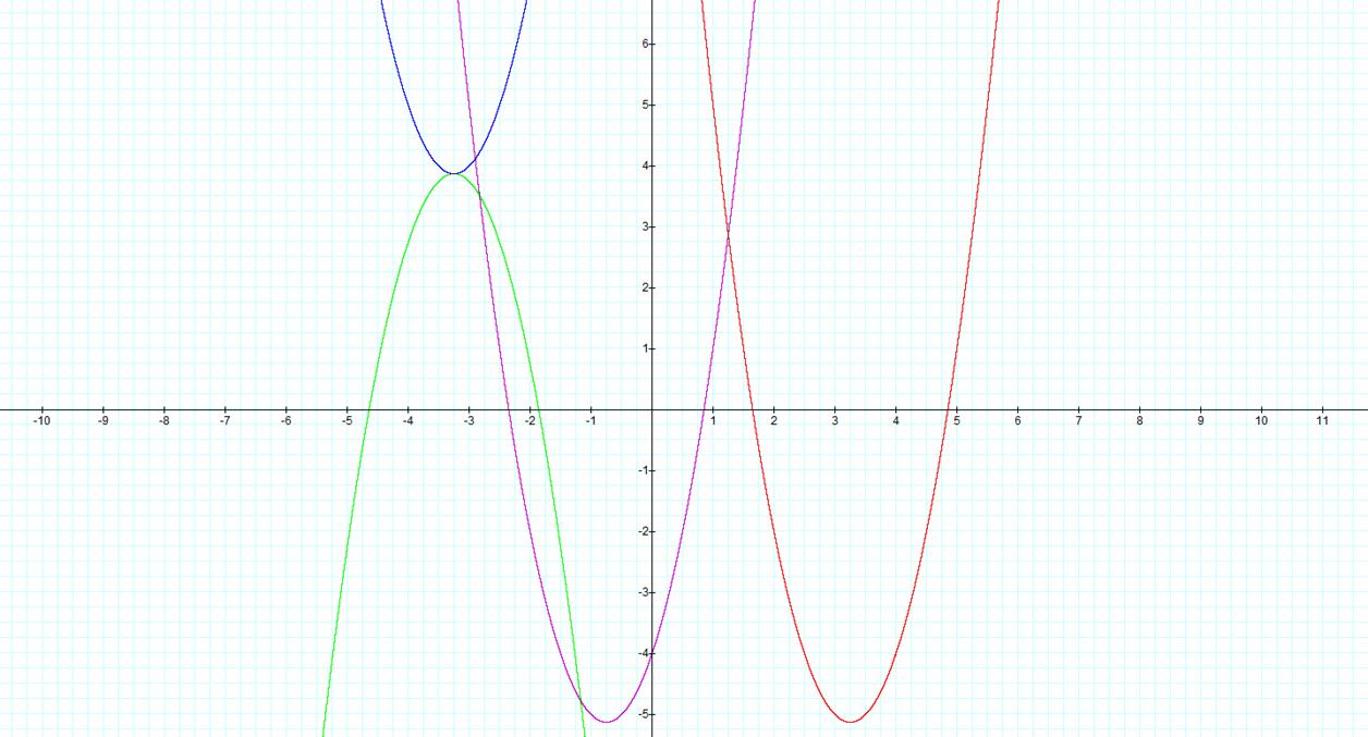
Figure 5-
Solutions to part ii and iii
Conclusion:
The most important things to take from this exploration are the
transformations that take place on a quadratic equation. If we know what adding
a coefficient, adding a value of x or adding a constant to the parent function
of ![]() does we can graph the equation quite simply. The following is
a summary of the findings of this exploration.
does we can graph the equation quite simply. The following is
a summary of the findings of this exploration.
Given the general quadratic equation![]() :
:
![]() shrinks the graph
shrinks the graph
![]() stretches the graph
stretches the graph
![]() stretches the graph and flips it concave down
stretches the graph and flips it concave down
![]() shrinks the graph and
flips it concave down
shrinks the graph and
flips it concave down
a>0 & a<0, b>0 vertex moves by 
a>0 & a<0, b<0 vertex moves by 
c>0 shifts the vertex up by c
c<0 shifts the vertex down by c