Fun With Quadratics

By Brandie Thrasher

Lets begin by examining the graph

y = ax²

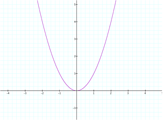
It looks as if we have our basic parabola. What exactly is a parabola?

Well, a parabola is a U-shaped curve for a point known as the focus and a line (not through the focus) called the directrix. The parabola is a locus of points, where the distance to the focus is equivalent to the distance to the directrix.

The standard form for a parabola is

y = a (x – h)² + k

But the general form (that most people recognize) is

y = ax² + bx + c

Lets see what happens to our parabola if we change our value for a (also known as our coefficient)

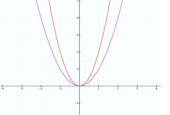
Our new parabola (in red) is the equation y = 2x². Looks as though this graph is slightly more narrow than or original equation, but why?

Let’s use a table and compare potential values

For this table, a = 1

x	ax^2	y
-2	(1)(-2)^2	4
-1	(1)(-1)^2	1
0	(1)(0)^2	0
1	(1)(1)^2	1
2	(1)(2)^2	4

x	2x^2	y
-2	(2)(-2)^2	8
-1	(2)(-1)^2	2
0	(2)(0)^2	0
1	(2)(1)^2	2
2	(2)(2)^2	8

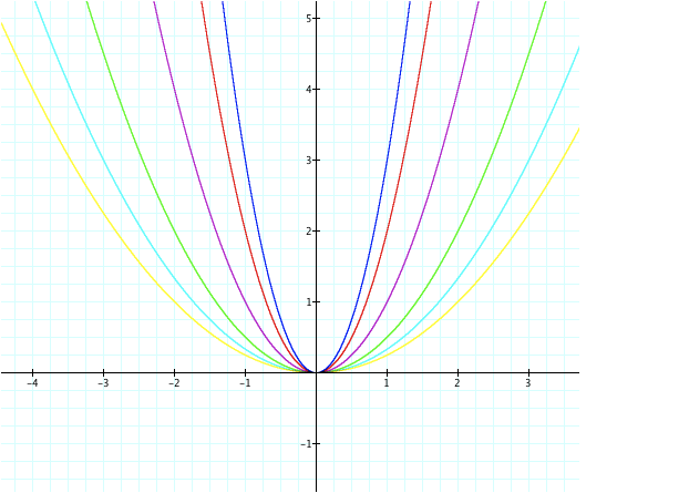
With our two tables we can analyze our values for y. It looks as though the distance between the y values is greater in the second chart (even as the actual distance increases), than the values in the first chart. This increase in distance is what causes the second graph to appear narrower. As our coefficient increases (is bigger than 1), or distance between values will continue to increase. How will y = 3x² appear on our graph?

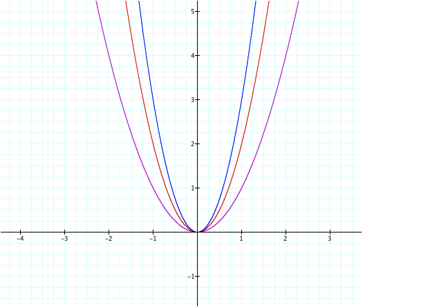
Here it is in blue (y = 3x²), and it is narrower than the first two. Looks good!!! But, what about coefficients less than 1 (but greater than zero), how would they impact our graph?

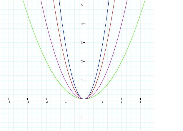
The green graph represents y = ½ x² and it appears to e wider than our original equation (in purple). Lets compare their charts

x	ax^2	y
-2	(1)(-2)^2	4
-1	(1)(-1)^2	1
0	(1)(0)^2	0
1	(1)(1)^2	1
2	(1)(2)^2	4

x	½ x^2	y
-2	(1/2)(-2)^2	2
-1	(1/2)(-1)^2	½
0	(1/2)(0)^2	0
1	(1/2)(1)^2	½
2	(1/2)(2)^2	2

In contrast to the previous example, these distances are less than those of the original equation. As our coefficients decrease (smaller than 1 but greater than 0) our parabola widens as the distance between the y values decrease.

Lets look at the graphs of y = ¹/₃ x² (in light blue) and y = ¼ x² (in yellow)

So, we’ve looked at coefficients greater than 1 and others that were greater than zero, but less than 1. What about coefficients less than zero?

Lets look at y = -2x² and compare it with y = 2x²

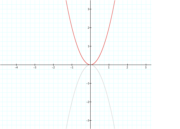
The two graphs appear to have the same shape, except the grey graph is facing downward, which means that all of its y values are negative. So we can see that our a value holds the same shape (or difference in distance between each value) whether negative or positive, but with the coefficient being negative our y values will all be negative.

As shown here for y = ax² and y = -ax²

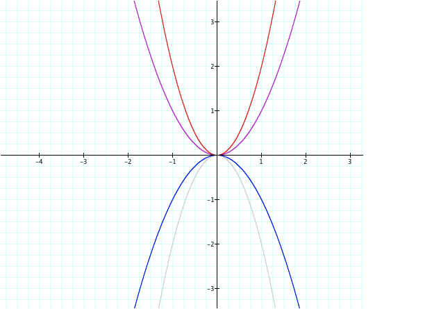
Lets see more!

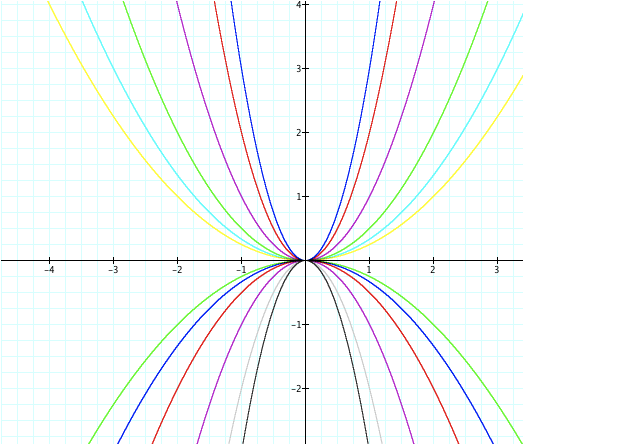
We can now generalize our graphs and know what they will look like with various coefficients

ANIMATION TIME!

Reference:

www.mathwords.com/p/parabola.htm

Return