
Assignment 1
Exploring Graphs
of Common Logs and Natural Logs
by
Jenny Johnson
The purpose of this exploration is to examine
the graphs of common logarithms (y = a log (bx)) and natural logarithms (y = a
ln (bx)).
What are the characteristics of the
graph of y = a log (bx)?
The
values for a and b alter the graph of a logarithmic function. When a = 1 and b
= 1, we have the standard equation y = log (x). This graph is illustrated below.
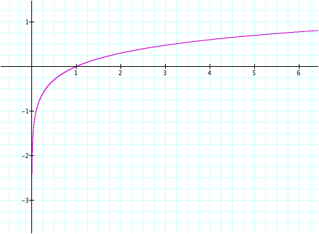
This
graph crosses the x-axis at one point, x = 1. It appears that it never crosses the y-axis. Instead, the log curve comes closer and
closer to the y-axis as the x-value decreases. We call the y-axis a vertical asymptote of the curve since
the distance between them approaches zero as the y-values approach negative
infinity. The log graph also
appears to continue increasing as x increases. What happens as x becomes arbitrarily large? Is there a horizontal asymptote of the
curve as well? Let’s zoom out on the graph to see what happens as x becomes larger.
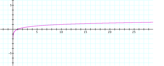
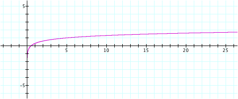
It
is clear from this graph that log (10) = 1. This makes sense since the base of the logarithm is 10, and
10¹= 10. As x increases, the y values continue to increase.
Will they approach a certain value?
Will the graph ever reach 2? Let us zoom out on the graph even further.
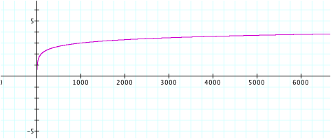
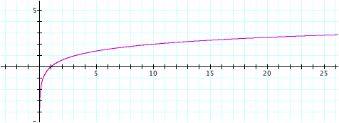
The
x increases, the curve does reach 2, then 3. Will it ever reach 5?
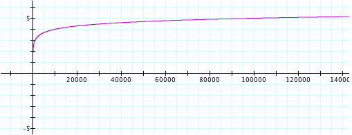
The
curve does reach 5. As x
increases, y will continue to increase.
Thus, we can safely say there is no horizontal asymptote. The domain of the graph y = log (x) is
therefore (0, ∞)
and the range of the graph is (-∞, ∞).
The x-intercept is located at x = 1, there is no y-intercept, and there
is a vertical asymptote at x = 0.
What happens to the common log graph
with varying values of a?
Let us first look at the graph when a = 2, y = 2 log
(x).
The
graph looks very similar to that of y = log (x). The graph still has an x-intercept when x = 1, the y-axis is
still a vertical asymptote, and the y-values increase as x increases. The only difference appears to be that
the y values increase at a faster rate as the x values increase. By watching a video file of the graph
as a ranges from 0 to 10, we can see
that the one feature of the graph that changes with a is the steepness of the
curve. As a increases, the curve
becomes steeper.
Let
us look at the graph when a is negative.
This video file shows the graph as a
ranges from -10 to 10.
Negative values for a invert the graph so that y values decrease as x
increases.
What happens to the common log graph
with varying values of b?
Let
us first look at the graph when b = 2, y = log (2x).
This
graph also looks very similar to the graph of y = log (x). The y-axis is a vertical asymptote and
the y-values increase as x increases.
It appears that the slope of the graphs are the same. The one difference observed is that the
x intercept occurs when x = ½. My conjecture is that the x-intercept
will occur when x = b/2. Let us explore this conjecture with a movie file with
b ranging from 0 to 10.
It
appears my conjecture is right.
The x-intercept will always occur when x = b/2. If this is true for all values of b,
then negative values of b should occur on the negative x-axis. This movie file shows the graph as b
ranges from -10 to 10.
We
see that the graph of y = log (-bx) is the reflection in the y-axis of the
graph of y = log (bx).
In
summary, changing the constant a in the graph of y = a log (bx) keeps
everything the same in the log graph except the slope of the curve. Changing the constant b changes the
x-intercept of the graph such that the intercept will occur when x = b/2. Certain features of the graph of the common
logarithmic function stay constant no matter how we alter a and b. The y-axis is always a vertical
asymptote of the graph. The range
of the graph is always (-∞, ∞).
What are the characteristics of the graph of the
natural logarithm y = a ln (bx)?
The
values for a and b alter the graph of a natural logarithmic function. When a =
1 and b = 1, we have the standard equation y = ln (x). This graph is illustrated below.
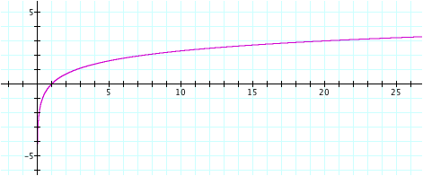
This
graph crosses the x-axis at one point, x = 1. It appears this graph also has an asymptote when x = 0. As we observed with the graph of y =
log (x), y will continue to increase as x increases. Thus, the domain of this graph is also (0. ∞) and the range
is (-∞, ∞). The only difference
between this graph of y = ln (x) and that of y = log (x) is that this graph
increases at a faster rate as x increases. Also, we know that ln (e) = 1 since the base of a natural log function is always e,
and e¹= e. We
can see on the graph that y = 1 when x is a little smaller than 3. This is a good approximation of e.
What happens to the graph of y = a ln(bx) with varying
values of a?
Changing
the value of a will likely change the slope of the graph as it did with the
regular log graph. Let us examine
a video of the graph as a ranges from -10 to 10.
We
see that the x-intercept stays at x = 1 and the y-axis is still a vertical
asymptote of the graph. The only
change is that the slope of the curve increases as a increases.
What happens to the graph with varying values of b?
Changing
the value of b will likely change the x-intercept of the graph as it did with
the graph of y = a log (bx). Let us examine a video of the graph as b ranges
from -10 to 10.
The
x-intercept will always occur when x = b/2.We see that
the graph of y = ln (-bx) is the reflection in the y-axis of the graph of y =
ln (bx).
From
the pictures and video files, it is clear that the parameters a and b do affect
the graphs of y = a log (bx) and y = a ln (bx).
How do the graphs of the common logarithm and natural
logarithm compare?
Let us graph the functions y = a log (bx) and y = a ln
(bx) on the same axes with a = b = 1.
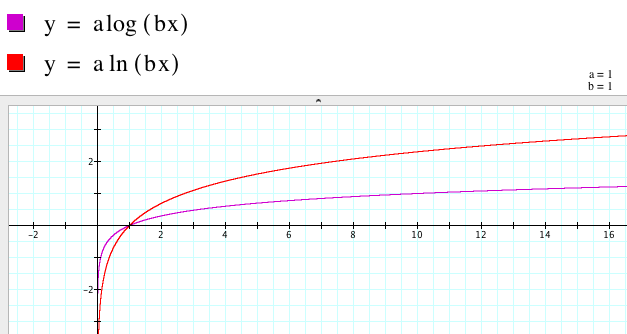
Now let’s graph them
when a = 2, b = 3.
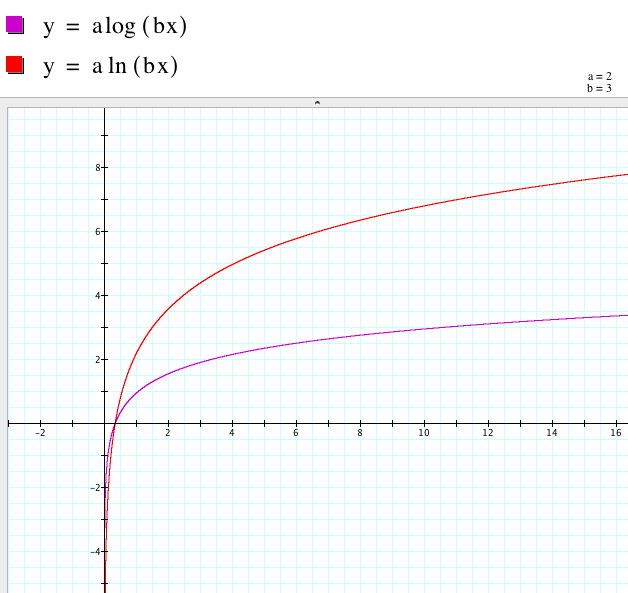
Now
it is clear that the two logarithmic graphs are similar curves with the same
x-intercept and vertical asymptote.
The major difference seems to be that the y-values in the natural log
graph increase at a faster rate than the y-values for the common logarithm
graph.
So, why do we need two different logarithmic
functions?
The
common logarithmic function uses 10 as the base of the logarithm. This function is useful for situations
like compound interest, the Richter scale, decibel levels, and the exponential
growth of a population.
The
natural logarithmic function uses the irrational constant e (euler’s constant
– 2.71818) as the base of the logarithm. This function is useful for situations in calculus,
statistics (for lines of best fit), and engineering.
Thus,
each one is useful in distinct situations.
How does the common logarithm y = a log (bx) connect
to its exponential function y = a (10bx)?
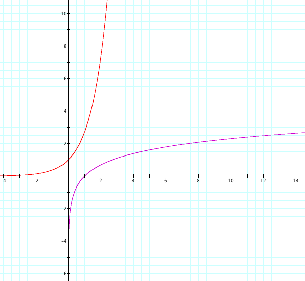
Let’s graph the common logarithm and its related
exponential function on the same axes.
It appears that the
common log graph is a reflection of the exponential function in the line y =
x.
How does the natural logarithm y = a ln (bx) connect
to its exonential function y = a (ebx)?
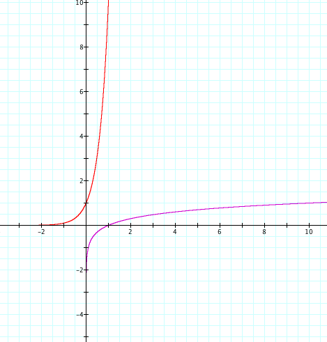
Let’s graph both of
them on the same axes with a = b = 1.
The
natural log graph is also a reflection of its related exponential function in the
line y = x.