Roxanne Kerry

For this third write-up, I decided to explore quadratic equations in a very different way that would typically be done – by changing the plane in which you graph the equations! This is an approach which, if explained well enough to high school students, could help them understand more about roots and quadratic equations in general. We will take a graphical approach, but, unlike the typical case in which we graph a basic function of ax²+bx+c = y, and vary a, b, and c in different explorations, we can instead graph this in various planes! Rather than graphing in the xy plane, we can, for example, graph in the xb plane, or in the xa plane, or even in the xc plane.

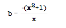
Now how in the world will we do this, and furthermore, how can this be done in a way in which high school students would understand and maybe even be able to do themselves? Initially, it took me a little while too to figure this out. Eventually, I came to the conclusion that when graphing in the xy plane, y is the variable solved for and x is the variable being used in the equation. If we want to graphically consider this while using the xb plane, we simply need to solve the equation for b. So, by setting y=0, x²+bx+1=0 becomes

On a graphing program such as Grapher (what I used), you cannot change the axes in which you graph, so I instead set the equation I found equal to y, set y equal to a parameter, and let the parameter vary and represent b. In the animation below, you will see the horizontal line as b as it varies, and the graph being the graph we found.

As you will notice, there are some places in which the graph is crossed twice by the horizontal line “b”, two places in which the graph is tangent to the horizontal line “b”, and some values for which the line “b” does not cross our other graph at all. These will represent the number of real roots in the equation. We can then see that when b is larger than 2 or smaller than -2, we have two real roots to the equation (because the line y=b crosses our graph twice). When b is equal to 2 or -2, we have one real root to the equation (because the line y=b lies tangent to our graph at these two points). Lastly, when b is between -2 and 2, we have no real roots to the equation (since the line y=b does not cross the graph at any points during this interval).

So what happens when we consider graphing in other planes to explore the same graph, say, the xc plane? We set up the graph similarly to how we did with the xb graph, by setting the equation equal to zero and solving for a, to get x²+x= c. We can model this by setting y= x²+x and taking y=c for varying c values. See animation below.

We can see here that y=c crosses our graph twice when c is greater than -.25, lies tangent to our graph when c is equal to -.25, and no times when c is less than -.25. This shows us that when c is greater than -.25 we will have two real roots, when c is equal to -.25, we will have one real root, and when c is less than -.25 there will be no real roots.

Now what about when we consider the xa plane? This one is slightly more difficult to solve for, but can be done.

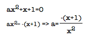
We can set our graph equal to y and a equal to y while letting a vary, to create an animation as follows:

This graph looks quite different but still can tell us the same information in terms of a. When a is greater than .25, it does not cross our graph, so there are no real roots. When a is between .25 and -.25 (not including -.25), it crosses our graph once, so we have one real root. When a is less than or equal to -.25, our graph is crossed twice, and so here we have two real roots.

So why use this seemingly complicated method of solving by graphing in various different planes? While it may not work for everybody, graphing in the various planes creates a very visual representation which can attach more meaning to students than formulas might. Also, this can be used if a student does not understand the standard way of finding roots, as this way it is easier to see what is going on.