
The Study
of Planes
By: Amanda Sawyer
In this investigation, we will study the
quadratic equation in the standard Cartesian coordinate system in the xy, xa, xb, and xc plane. We will determine what effects the a, b and c variable have on each
of these planes.
1.
THE XY PLANE
Let’s
first discuss the effects of a, b, and c in the xy plane. We can observe this change by changing each
coefficient. First, let’s look at what
happens when the a value changes. The next four equations were graphed with
their b and c values equaling zero.
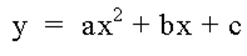
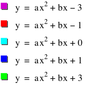
A Value
Changed in XY Plane
|
Equations |
Graph |
|
|
|
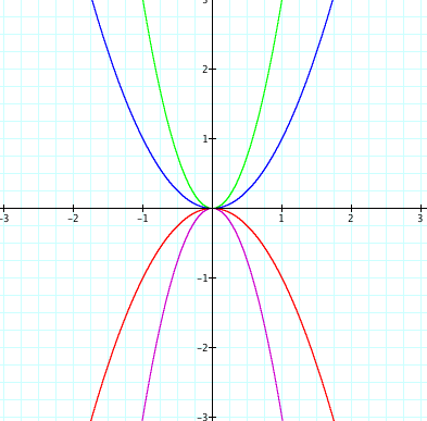
It is clear from this picture that if our a
value changes the concavity of our graph changes. When our a value
is positive, we will have a graph with both endpoints going toward positive
infinity. When our a
values are negative, the graphs endpoints will go towards negative
infinity. We also can see that the
larger the absolute value of our a
the more the graph is stretched.
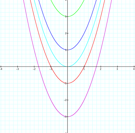
Now
let’s study what happens when our b values change in our
equation. The follow five equations were
used to study the relationship between each equation with the
a
value equaling one and the c value equaling zero.
B Value
Changed in XY Plane
|
Equations |
Graph |
|
|
|
It
is easy to see that this change in value moves our vertex for each graph, but
it does not change its concavity.
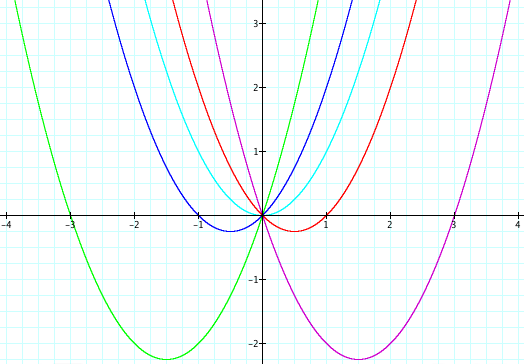
Our
last step in our xy plane is to study the
effects of the c value. When we allow a values to equal 1 and the b values to equal 0, we
will receive the following equations and graphs.
C Value
Change in the XY Plane
|
Equations |
Graph |
|
|
|
Again
we can see that this changes our vertices position in our graphs. When our b = 0, the c value represents the
y-intercepts of each of the five equations.
From this information, we can see what characteristic of our graph have
with a given a, b, or c value in our quadratic equation.
2. THE XB
PLANE
Now
that we know how our graph responds in our traditional XY plane, let’s study
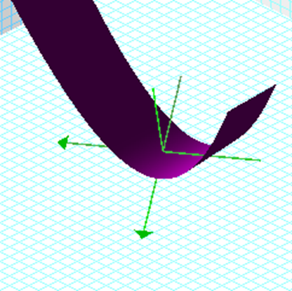
what happens when we graph equations in the XB plane. We can view this three dimensional realm
plane in the picture bellow.
The easiest way to visualize the xb plane is to
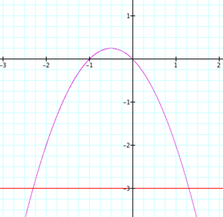
substitute b with y and graph it. We set the quadratic equal to zero to show
all the possible roots of b for our equation. When we graph this equation in the two
dimensional realm as in Figure 1, we can find the roots of x. When we draw a vertical line (b = 4
in green), we can find the roots of our equation from the intersection of these
two lines. In the graph below we see
that when we set a and c equal to one, we have
two possible roots for x at b = 4. These values are located x =
-.267949 and x = -3.73205.
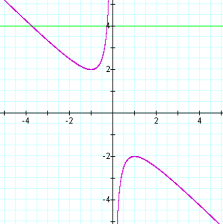
FIGURE 1
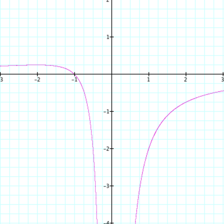
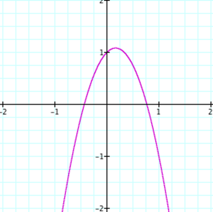
If we graph the equation the ax + 4x + c = 0 for a and c equaling 1 in the xy plane, we get the following graph. The x-intercepts of this graph are the roots
that we found in the above equation. As
you can see from Figure 2, the x-intercept is the points x = -.267949 and x =
-3.73205.
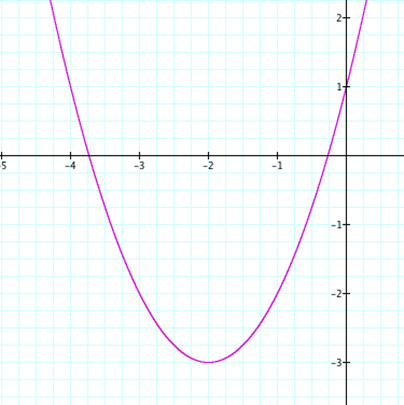
FIGURE 2
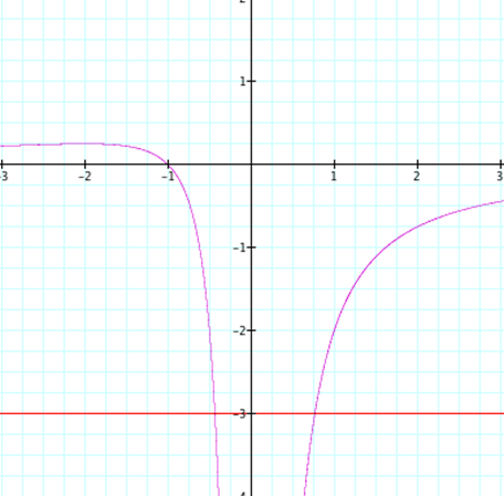
We can even overlap these graphs by putting the xb-plane
on top of the xy-plane:
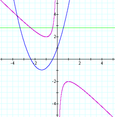
FIGURE 3
Notice
in Figure 3 how the points of intersection (green and purple lines) are exactly
above the intersection of the blue graph with the x-axis. From this information we can make some
generalization. Since our equation does
not exist in the xb plane between -2 and 2,
we do not have any x-intercepts at between those two points.
3.
THE XA PLANE and XC PLANE
We can now repeat this for both the xa plane
and the xc plane. As we can see from the table below, we can
again view the roots of our equations with any given a value in the xa-plane and any given c value in the xc plane.
|
|
XA PLANE |
XC PLANE |
|
3-Dimensional View |
|
|
|
2-Dimensional View |
|
|
|
For Solution of -3 |
|
|
|
XY Plane of Equation with
-3 |
|
|
We
can see from this information, that we can find any roots for any given a or c value. For example, we found the roots for a =
-3 and c = -3 in the graphs
above. Those intersections are the roots
in the xy plane.
4.
Conclusion
For
all of the above problems the values of the other two variables in the plane
were kept constant with a value of 1. If
we change the coefficients in all the above-mentioned planes, the graphs are
very difficult to view since each coefficients change in unison. This is an oversimplification because it is
rare for a = b = c with parabolas, to show all the planes and their
relationships to each other would require more than a mere 2 dimensions.
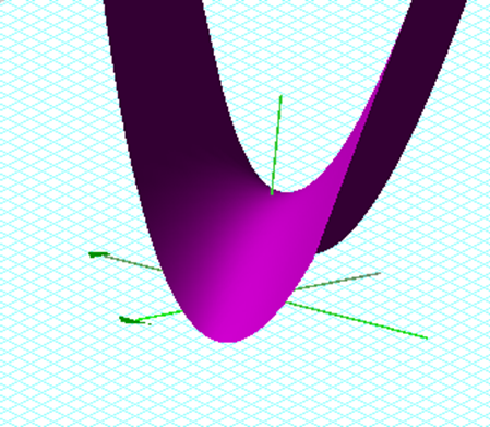
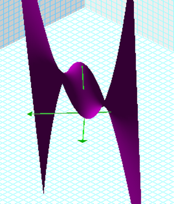
We
can view this change in the below graph were the value for a, b, and c
is equal to 0.8 in this case. In this
picture xb plane is light blue, xa plane is dark gray, and xc
plane is red. We can see that when your
value of these variables is close to one, there isn’t a root in the xa, xb, and xc plane.
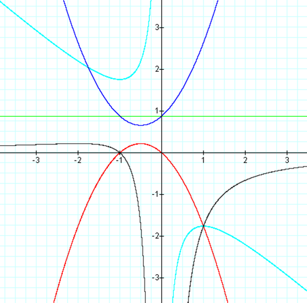
FIGURE 4
In this investigation, we say the different
relationships created by different planes.
By using this graphing technology to create the new planes, it was
easier to understand and explain these concepts to others.