Starbust Quadratics
Allyson Faircloth
For this write up we will be looking at the quadratic equation
when a is equal to 1. We also want to look at the equation in the x-b plane, so we will need to let b = y and explore within the x-y plane.
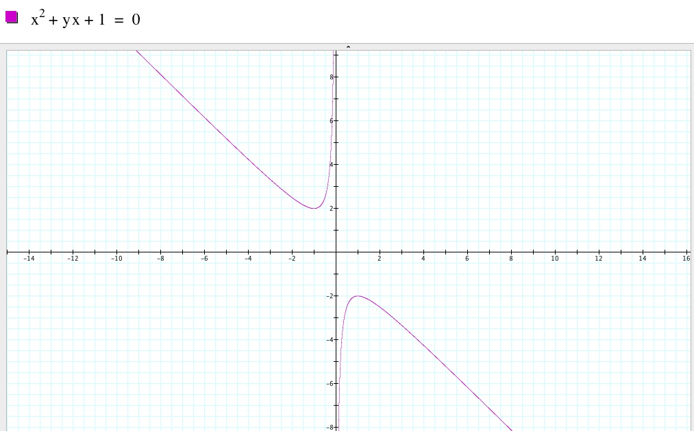
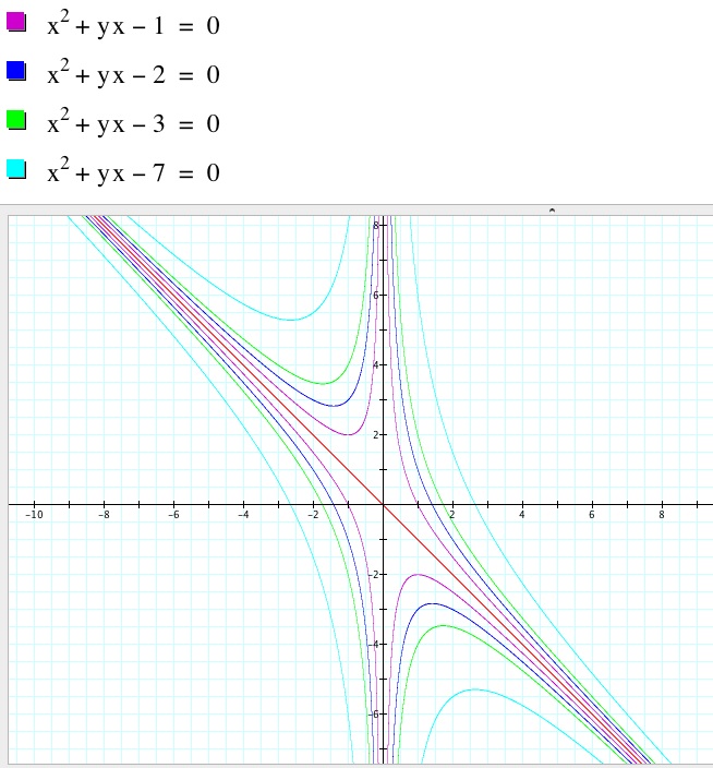
For the first equation, we will look atwhen c = 1.
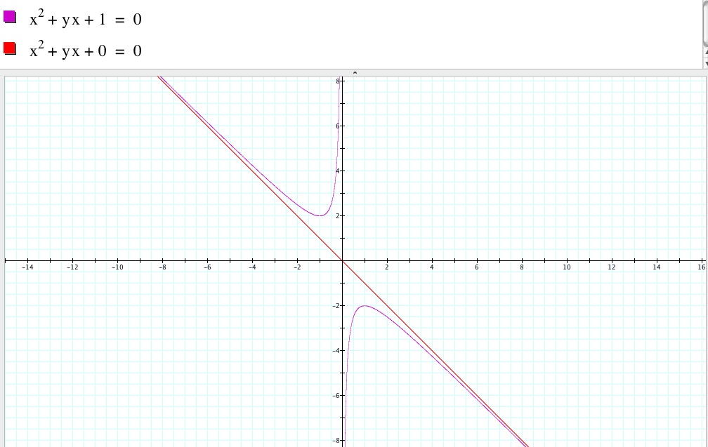
We can recognize a few things from the graph. First of all, the function is a hyperbola with one portion in the second quadrant and another portion in the third quadrant. Secondly, since the function is a hyperbola there will be two different asymptotes. By looking at the graph, it seems that one asymptote is the x-axis, yet it is hard to determine the second asymptote just by looking at the graph.Let’s take a look at when c = 0.
We have found our other asymptote! This asymptote can also be written as x = -y.
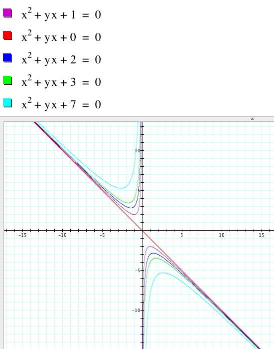
Let’s take a look at a few more graphs with positive c values.
These graphs seem to be between each of the graphs before them and still have the same asymptotes.
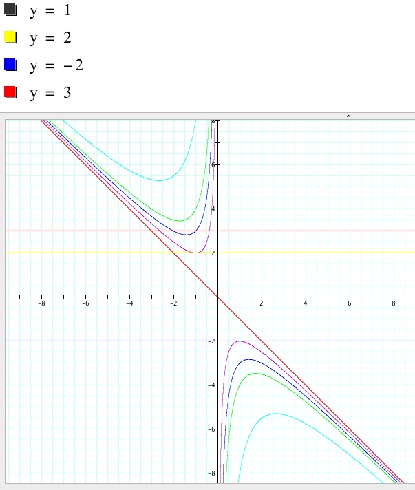
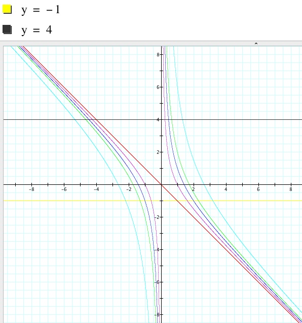
Now let’s take a look at another aspect. Below are the graphs from above along with the graphs of some horizontal lines.
Since the line y = 3 is crossing the graph oftwice, the two intersection points are the two real roots of the original function where y = 3. Now let’s look at y = 1. This graph does not cross the function’s graph. Since there are no intersections, then there are no real roots.
Where will there be one real root? The only way there will be one real root is when the horizontal line is tangent to the vertex. As we can see, the graph of y = 2 is a tangent line to the vertex and shows us the one real root. However, there will also be one real root with the graph of y = -2 which is the tangent line to the vertex in the fourth quadrant.
Therefore, when c is positive for
If we look specifically at our first graph (
Now let's take a look at when c is equal to a negative number.
We can see that our graphs have reflected across the asmpytote x = -y. What do we know about the roots of the equation when c is a negative value?
By looking at the graph above, we can see that for any value of y there will always be two real roots for the original function with a negative value for c.
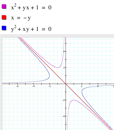
Now what will happen if we swap y and x so that we have
. Let’s try and see.
The graph has been reflected over the asymptote x = -y.
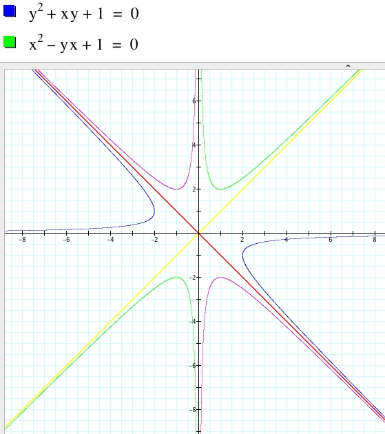
We saw that a negative c value reflected the graph across the asymptote –y = x. But how can we get our graphs into the first and third quadrants? Let's try a negative value for our b of
We now have our original equation in the first quadrant with the asymptotes x = 0 and y = x. Now if we swap y and x in our equation, we will reflect this new graph in the first quadrant across the y = x asymptote by changing our b value foror x into a negative value.
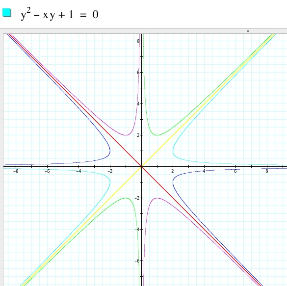
Now that all of our different alterations of the equation are together, we have a very interesting design which reminds me of some kind of starburst.In conclusion, if we had begun with our equation
1. Reflect across the y-axis
2. Reflect across the line x = -y
3. Reflect across the x-axis
4. Reflect across the line y = x
5. Reflect across the y-axis
6. Reflect across the line x = -y
7. Reflect across the x-axis.
Return