Linear Function Parameters

by: Maggie Hendricks

Linear Functions can be thought of as being written in the form y = a(x-k)+h, for parameters a, k, and h. In this exploration, we will take a look at what effect each of these three parameters have on the graph of a linear function. To begin, let's hold a equal to 1, k equal to 0, and look at varying values of h. Below you will see the graph of y = x + h, for 9 cases: when h = -4, -3, -2, -1, 0, 1, 2, 3, and 4.

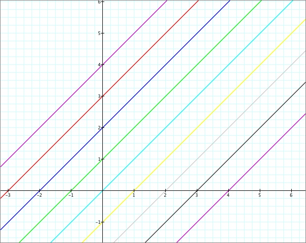
The line at the far right (the second pink one) is the graph for the case when h is equal to -4, and as you move to the left, each line shows the case for -3, -2, -1, 0, 1, 2, 3, and 4, respectively. We can see that the parameter h seems to effect the x-intercept of our function (in these cases, the x-intercept is equal to additive inverse of the parameter h). Now let's take a look at a graph that shows changes in the parameter h as a movie.

We see the constant movement of the linear function as the parameter h shifts from -4 all the way up to +4. It is helpful to see it in this manner so as to avoid the misconception that the function only exists at integer values of h and hops from each of the lines shown in the first picture to the next. The movement we see here reminds us that the parameter h can take on any real number value, and non-integer values do not change the expected behavior of our function.

Now let's take a look at what happens when we change the parameter k. Taking the same 9 functions from before, let's see what happens to our graph if we let k be equal to 2. See the graph below for a visual.

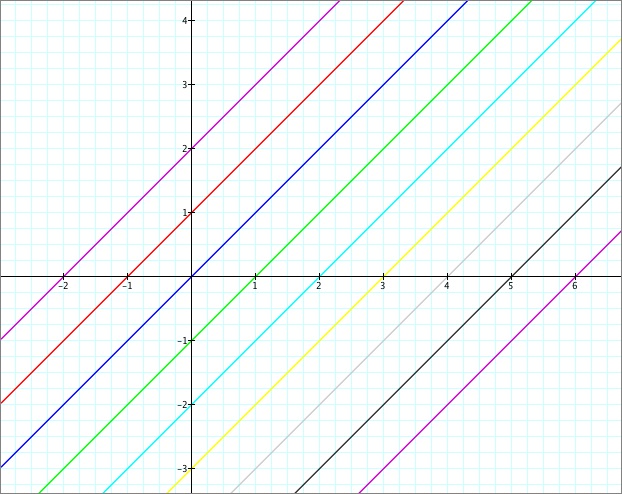
We can see that the only thing that has changed here is that the x-intercept is no longer equal to -h. All of our x-intercepts have shifted over to the right by two (or the parameter k). This makes sense algebraically, since we can simplify the function

y = (x-2)+(-4) to read y = x+(-6), so we would expect the x-intercept to take place at 6 instead of 4. Let's take a look at this function as we constantly change h. See the movie below.

Again, seeing the function in constant motion helps us remember that it takes on functional values when the parameter his a non-integer as well as when it is a whole number. Finally, let's take a look at changes in the parameter a when k is held constant at 2 and h is held constant at zero. See the graph below for a visual of what the function looks like when a is equal to -4, -3, -2, -1, 0, 1, 2, 3, and 4.

We see here that the parameter a effects the overall slope or steepness of our function. When a is positive, we see that the graph increases in value from right to left, and when a is negative the graph decreases in value from left to right. A special case occurs when a is equal to zero. The function takes on a constant value of zero in this case and forms a line across the x-axis. We can also look at changes in this parameter as it moves constantly from -4 to +4.

Again, this fluid movement and change in the parameter allows us to dynamically see that when k and h are held constant, the function rotates around the fixed point of (2,0), only changing in steepness or slope as a changes.

Click here to return to Maggie's homepage.