Untitled Document

The following is a table of data with the independent variable as minutes and the dependent variable is temperature. The data is was collected by measuring the temperature of water every minute for 30 minutes. The water is in the process of cooling, but the ambient temperature is not provided. For this exploration, we will use a spreadsheet in Excel to construct an equation to predict the temperture.

Minutes 0	Temperature 212
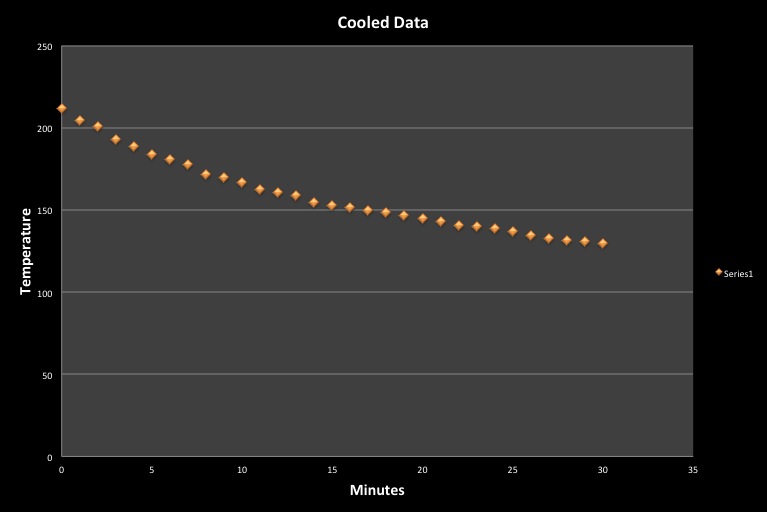
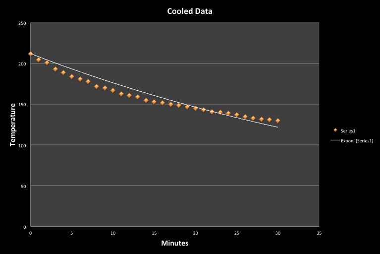
1	205
2	201
3	193
4	189
5	184
6	181
7	178
8	172
9	170
10	167
11	163
12	161
13	159
14	155
15	153
16	152
17	150
18	149
19	147
20	145
21	143
22	141
23	140
24	139
25	137
26	135
27	133
28	132
29	131
30	130

Here is a graph of the raw data:

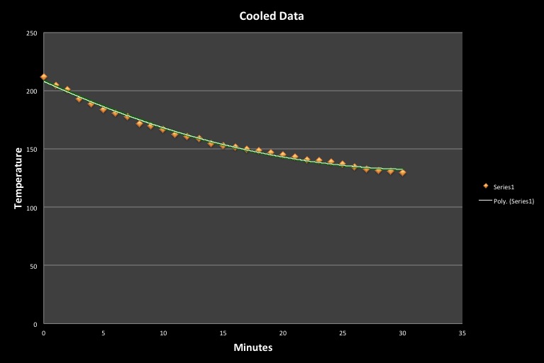
At my first attempt of finding an equation, I tried to use Excel to fit an exponential equation to the data and setting the y-intercept to y = 212. The line didn't seem to fit well at all so then I tried using Excel for a polynomial fit (of order 2), which appeared to fit very well.

Next I found the predicted temperatures for all the times and found a measurement of error by calculating the sum of the errors squared. After doing this, it appears that the quadratic equation fit the best.

Exponential Equation Prediction:

SSE = 40.55

Quadratic Equation Prediction:

SSE = 3.04

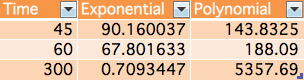
Then I tried using each equation to predict the temperature at 45, 60, and 300 minutes.

Clearly, the water temperature should not increase if it's just sitting in a room with a constant ambient temperature, so the quadratic equation is out. Also, the temperature should not go down to 0 degrees because the data appears to be leveling out near 120 degrees. Then I realized that Excel's best fit for an exponential equation was in the format y = ae^(-bx). So the prediction equation always has a limit of 0.

We have to take into account that the data appears to have a limit of 120.

So the equation should be in the format y = ae^(-bx) + 120.

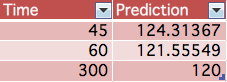
The equation Excel first gave was y = 212e^(-.019x). In order to add a limit of 120, but keep the y-intercept at 212, we have to subtract 120 from 212 for our new coefficient. Now we have y = 92e^(-.019x) + 120. Using excel, we can change the value of b and see the resulting predictions and SSE immediately. From a process of trying different values for b and watching the SSE rise and fall, the resulting equation is y = 92e^(-.068x) +120. Here is the data using this equation:

SSE = 1.30

The SSE is a lot smaller and I'm sure with a little more trial and error, it would be possible to get this value even closer to 0. But these predictions also seem a lot more realistic if the ambient temperature is 120 degrees.