Back in the first investigation we looked at
figure eights, also known as lemniscates. We decided that the
equation for a lemniscate with foci at (-a, 0) and (a, 0) was
![]() . Now we are going to revisit the
lemniscate but we are going to look at it using a different kind
of mathematical tool. In the last investigation we learned how
to plot using parametric equations instead of the traditional
rectangular coordinates. Now we are going to learn to plot another
way, using polar coordinates. Once we understand what polar coordinates
are we can go back and look at how the figure eight can be explored
using our new knowledge.
. Now we are going to revisit the
lemniscate but we are going to look at it using a different kind
of mathematical tool. In the last investigation we learned how
to plot using parametric equations instead of the traditional
rectangular coordinates. Now we are going to learn to plot another
way, using polar coordinates. Once we understand what polar coordinates
are we can go back and look at how the figure eight can be explored
using our new knowledge.
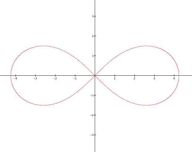
In the last investigation we learned how we can represent graphs using parametric equations. The point of being able to use parametric equations was to be able to answer questions more easily than if we were using rectangular coordinates. Polar coordinates play a similar role. They allow us to work with equations and plot them more easily than if we tried to use rectangular coordinates. The way we think of a point on a graph with rectangular coordinates is (x, y) where x is the horizontal distance from the origin to the point and y is the verticle distance from the origin to the point.
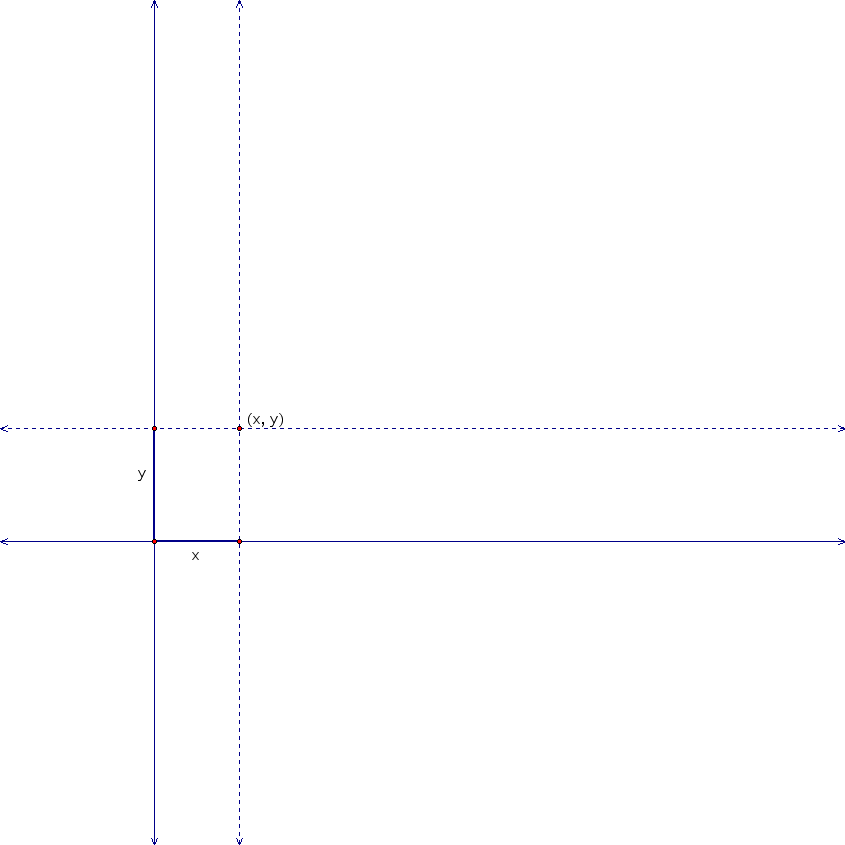
Now we are going to think of the point in a different way. Imagine drawing a line segment from the origin to our point of interest. The two things we are going to look at is the length that line segment, which we denote by r, and the angle that segment makes with the positive half of the x-axis.
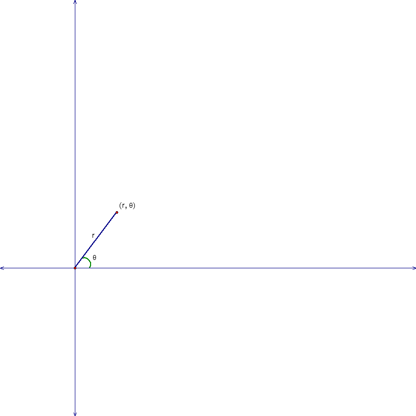
It should make since that because we are representing the same point two different ways that there should be a relationship between the rectangular coordinates and the polar coordinates. Indeed, there is. Let's combine the important aspects of the point for the two coordinate systems onto one picture.
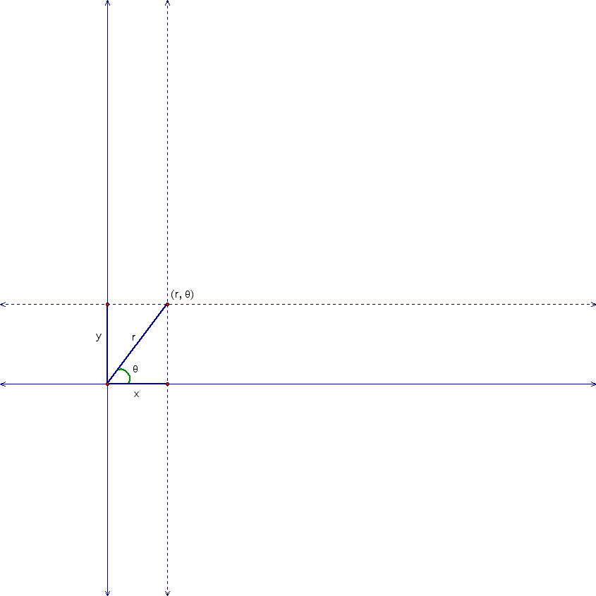
We are going to take the verticle line segment, y, and shift it to the right so that we are working with a triangle.
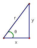
Now let's use our definitions of sine and cosine to find a relationship between the variable in this picture.


Solve for x and y to see how polar coordinates and rectangular coordinates are related.
As you can see, we can go back and forth between rectangular coordinates and polar coordinates if need to. Or we can just choose which coordinate system is most beneficial to us during any given problem.
Let's return to the problem of the lemniscate and look at it from the point of view of polar coordinates. In rectangular coordinates the equation was
Using what we just found we can convert this to polar coordinates using substitution.
I ask you, which looks nicer to work with ![]() or
or ![]() ?
?
Assume for the moment that a=1. Let's plot
a few points so that you can see how to work with polar coordinates.
We are going to plot for various ![]() as
the table beneath dictates.
as
the table beneath dictates.
| |
0 | 2 |
3 |
5 |
7 |
5 |
4 |
3 |
5 |
7 |
11 |
2 |
|||||
| 2 |
0 | 2 |
4 |
3 |
5 |
2 |
7 |
5 |
8 |
3 |
10 |
7 |
11 |
4 |
|||
| cos(2 |
1 | 1/2 | 0 | -1/2 | -1 | -1/2 | 0 | 1/2 | 1 | 1/2 | 0 | -1/2 | -1 | -1/2 | 0 | 1/2 | 1 |
| 2cos(2 |
2 | 1 | 0 | -1 | -2 | -1 | 0 | 1 | 2 | 1 | 0 | -1 | -2 | -1 | 0 | 1 | 2 |
| r | 1 | 0 | DNE | DNE | DNE | 0 | 1 | 1 | 0 | DNE | DNE | DNE | 0 | 1 |
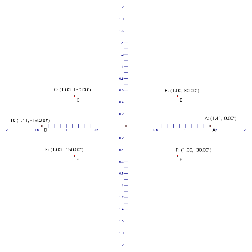
Since the origin was plotted several different
times its coordinates for left out so that the picture did not
become too cluttered. You can imagine connecting these points
and getting the lemniscate. If you can't see that then try adding
more points to the graph and plotting those. Another small change
in our picture is that ![]() is measured in
radians in our chart and in degrees in our picture. If you do
not feel comfortable with that then translate our chart on paper.
This is good practice and you should be able to go from radians
to degrees and back with little effort.
is measured in
radians in our chart and in degrees in our picture. If you do
not feel comfortable with that then translate our chart on paper.
This is good practice and you should be able to go from radians
to degrees and back with little effort.
Now that we have the equation for the lemniscate in polar coordinates let's explore what happens when we vary parts of this
equation.
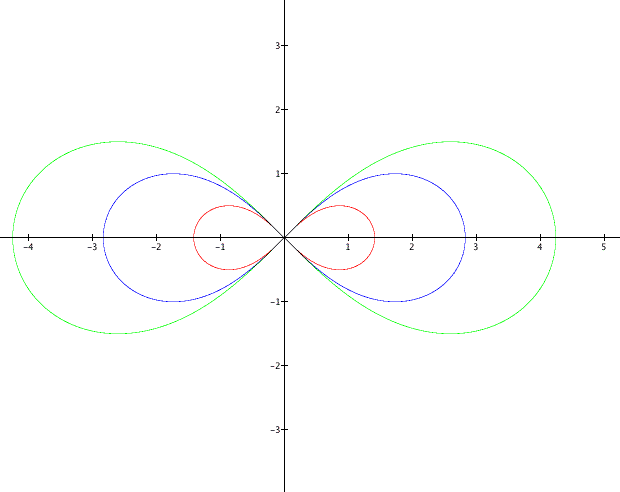
Since the range for ![]() is -1 to 1 it would make sense that changing the value for a would
change the range for
is -1 to 1 it would make sense that changing the value for a would
change the range for ![]() , which is from
0 to
, which is from
0 to ![]() (why is the lower limit 0 instead
of -
(why is the lower limit 0 instead
of -![]() ?). That means the lemniscate will
be streched out when a is changed. The picture below confirms
this. It is a lemniscate that has the form
?). That means the lemniscate will
be streched out when a is changed. The picture below confirms
this. It is a lemniscate that has the form ![]() when a=0,
1,
2
and 3.
when a=0,
1,
2
and 3.
Now let's think of the general form of a lemniscate
as being ![]() . What happens when we change b?
This is harder to predict so let's just see what kind of pictures
we get when b=-2, 0, 2.
. What happens when we change b?
This is harder to predict so let's just see what kind of pictures
we get when b=-2, 0, 2.
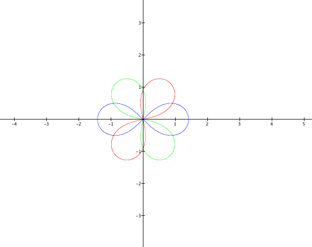
It appears to be spinning the graph. That happens
because at any given ![]() we are getting
different radii lengths. Still confused? Rewrite our equation
for the lemniscate by using additive angle formulas.
we are getting
different radii lengths. Still confused? Rewrite our equation
for the lemniscate by using additive angle formulas.
Can you see that if our parent equation was
then when we add b on the inside we are essentially
taking our old ![]() and multiplying
it by the constant
and multiplying
it by the constant ![]() and then adding
to that the new new value for
and then adding
to that the new new value for ![]() . Now
knowing what you do about values for the trigonimetric functions
at various
. Now
knowing what you do about values for the trigonimetric functions
at various ![]() values see if you can understand
why we get the pictures above. Given a value for b, can you predict
how the lemniscate will look? Notice that if b equals 2
values see if you can understand
why we get the pictures above. Given a value for b, can you predict
how the lemniscate will look? Notice that if b equals 2![]() or any integer multiple of 2
or any integer multiple of 2![]() then
sin(b)=0 and cos(b)=1. Then since
then
sin(b)=0 and cos(b)=1. Then since
we get that
In other words, adding b inside makes no difference
to the graph when b is a multiple integer of 2![]() .
.
There are so many things that can explored
with this problem that there just isn't enough time. What happens
if cos(2![]() ) is replaced with sin(2
) is replaced with sin(2![]() )
or tan(2
)
or tan(2![]() )? What about if we change it to
)? What about if we change it to
![]() ? What happens if 2
? What happens if 2![]() becomes 3
becomes 3![]() or -5
or -5![]() ? What
if we add values to the end of our polar coordinate equation so
that the general form looks like
? What
if we add values to the end of our polar coordinate equation so
that the general form looks like ![]() or
or
![]() ? Which c values result in the
figure eight and which ones cause our graph to fall apart? How
can these be predict? Why are they behaving in such a way? So
much math, so little time.... Have fun exploring.
? Which c values result in the
figure eight and which ones cause our graph to fall apart? How
can these be predict? Why are they behaving in such a way? So
much math, so little time.... Have fun exploring.