
Erin Mueller
Excel and APY
Excel can
be used to explore many areas of mathematics including functions and graphs.
Excel is a great tool for exploring annual percentage yields. When money is
deposited into a savings account, this money will accrue interest over time.
This means you will have more money than when you started (assuming you did not
withdraw any) without ever depositing any. The first deposit made into your
account is called the principal amount or the beginning amount. Your interest rate
will vary depending on the length of time the account is open (will depend
entirely upon yourself) and the type of account chosen. Accounts known as
certificates of deposit (CD) will require you to keep your first deposit in the
bank for a certain length of time. You are not allowed to touch this money
while it is in the bank. However, interest rates on these types of accounts
tend to be good and can range from 2% - 6% annual interest rate. Other factors
include how long you tend to keep the account open and how many times per year,
interest is accumulated. It may be yearly, semi-annually, or quarterly,
depending on the bank. The Excel chart below shows how much money will be accrued
after 10 years, in which the interest is compounded quarterly (4 time per
year), and the interest rate is 1.99%. The chart shows how much money will be accrued
based on the principal while the length of time, interest rate, and number of
times interested is compounded are kept constant.
|
Principal |
Interest Rate (Annual) |
#Of Times Interest is Compounded
per Year |
# Of Years |
Total Amount in Account After N
Years |
|
|
P |
r |
q |
n |
A |
|
|
2000 |
0.199 |
4 |
10 |
3250.04 |
|
|
2500 |
0.199 |
4 |
10 |
4062.55 |
|
|
3000 |
0.199 |
4 |
10 |
4875.06 |
|
|
3500 |
0.199 |
4 |
10 |
5687.57 |
|
|
4000 |
0.199 |
4 |
10 |
6500.08 |
|
|
4500 |
0.199 |
4 |
10 |
7312.59 |
|
|
5000 |
0.199 |
4 |
10 |
8125.10 |
|
|
5500 |
0.199 |
4 |
10 |
8937.61 |
|
|
6000 |
0.199 |
4 |
10 |
9750.12 |
|
|
6500 |
0.199 |
4 |
10 |
10562.63 |
|
|
7000 |
0.199 |
4 |
10 |
11375.14 |
|
|
7500 |
0.199 |
4 |
10 |
12187.65 |
|
|
8000 |
0.199 |
4 |
10 |
13000.16 |
|
|
8500 |
0.199 |
4 |
10 |
13812.67 |
|
|
9000 |
0.199 |
4 |
10 |
14625.18 |
|
|
9500 |
0.199 |
4 |
10 |
15437.69 |
|
|
10000 |
0.199 |
4 |
10 |
16250.20 |
|
|
10500 |
0.199 |
4 |
10 |
17062.71 |
|
|
11000 |
0.199 |
4 |
10 |
17875.23 |
|
|
11500 |
0.199 |
4 |
10 |
18687.74 |
|
|
12000 |
0.199 |
4 |
10 |
19500.25 |
|
|
12500 |
0.199 |
4 |
10 |
20312.76 |
|
|
13000 |
0.199 |
4 |
10 |
21125.27 |
|
|
13500 |
0.199 |
4 |
10 |
21937.78 |
|
|
14000 |
0.199 |
4 |
10 |
22750.29 |
|
|
14500 |
0.199 |
4 |
10 |
23562.80 |
|
|
15000 |
0.199 |
4 |
10 |
24375.31 |
|
|
15500 |
0.199 |
4 |
10 |
25187.82 |
|
|
16000 |
0.199 |
4 |
10 |
26000.33 |
|
|
16500 |
0.199 |
4 |
10 |
26812.84 |
|
|
17000 |
0.199 |
4 |
10 |
27625.35 |
|
|
17500 |
0.199 |
4 |
10 |
28437.86 |
|
|
18000 |
0.199 |
4 |
10 |
29250.37 |
We can
also see this data in a chart. The Principal amount represents the input
(x-axis) and the output is the Amount Earned (y-axis).
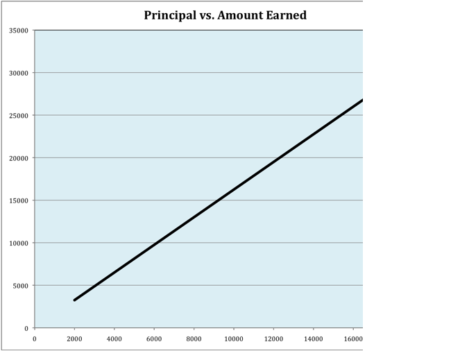
As we can
see, this is a linear function. Note that in this case, the interest rate
remains a steady 1.99%, the number of times compounded in a year remains 4
(quarterly), and the number of years the money is kept in the account remains
10. We can find the regression of our data as well as the r-square value using
Excel. Y=812.51x+2437.5 and r-square
= 1. The r-square value represents the association between x and y. In this
case, the data points accurately portray the linear regression function. Now
let’s look at what happens when the interest rate is isolated. Below is the
chart of data when the Principal is a constant $2,000, the interest is still
compounded quarterly, and the money is still in the account for 10 years. The
only variable changing is the interest rate.
|
Principal |
Interest
Rate (Annual) |
#
Of Times Interest is Compounded per Year |
#
Of Years |
Total
Amount in Account After N Years |
|
|
P |
r |
q |
n |
A |
|
|
2000 |
0.199 |
4 |
10 |
3250.04 |
|
|
2000 |
0.209 |
4 |
10 |
3328.28 |
|
|
2000 |
0.219 |
4 |
10 |
3408.20 |
|
|
2000 |
0.229 |
4 |
10 |
3489.85 |
|
|
2000 |
0.239 |
4 |
10 |
3573.26 |
|
|
2000 |
0.249 |
4 |
10 |
3658.45 |
|
|
2000 |
0.259 |
4 |
10 |
3745.47 |
|
|
2000 |
0.269 |
4 |
10 |
3834.35 |
|
|
2000 |
0.279 |
4 |
10 |
3925.12 |
|
|
2000 |
0.289 |
4 |
10 |
4017.82 |
|
|
2000 |
0.299 |
4 |
10 |
4112.49 |
|
|
2000 |
0.309 |
4 |
10 |
4209.16 |
|
|
2000 |
0.319 |
4 |
10 |
4307.87 |
|
|
2000 |
0.329 |
4 |
10 |
4408.65 |
|
|
2000 |
0.339 |
4 |
10 |
4511.56 |
|
|
2000 |
0.349 |
4 |
10 |
4616.62 |
|
|
2000 |
0.359 |
4 |
10 |
4723.88 |
|
|
2000 |
0.369 |
4 |
10 |
4833.38 |
|
|
2000 |
0.379 |
4 |
10 |
4945.15 |
|
|
2000 |
0.389 |
4 |
10 |
5059.25 |
|
|
2000 |
0.399 |
4 |
10 |
5175.71 |
|
|
2000 |
0.409 |
4 |
10 |
5294.57 |
|
|
2000 |
0.419 |
4 |
10 |
5415.89 |
|
|
2000 |
0.429 |
4 |
10 |
5539.71 |
|
|
2000 |
0.439 |
4 |
10 |
5666.06 |
|
|
2000 |
0.449 |
4 |
10 |
5795.01 |
|
|
2000 |
0.459 |
4 |
10 |
5926.59 |
|
|
2000 |
0.469 |
4 |
10 |
6060.85 |
|
|
2000 |
0.479 |
4 |
10 |
6197.84 |
|
|
2000 |
0.489 |
4 |
10 |
6337.62 |
|
|
2000 |
0.499 |
4 |
10 |
6480.22 |
|
|
2000 |
0.509 |
4 |
10 |
6625.71 |
|
|
2000 |
0.519 |
4 |
10 |
6774.13 |
Below is
the graph of the data.
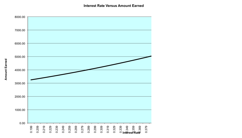
This
function looks exponential. The regression equation and correlation coefficient
for this graph is  .
.
This means
that if we plug a value for the interest rate in for “x”, the out put will be
our amount earned based on a $2,000 principal and ten year, quarterly return.
Next, we
can see what happens when we change the number of times interest is compounded
throughout the year.
|
Principal |
Interest
Rate (Annual) |
#Of
Times Interest is Compounded per Year |
#
Of Years |
Total
Amount in Account After N Years |
|
|
P |
r |
q |
n |
A |
|
|
2000 |
0.199 |
4 |
10 |
3250.04 |
|
|
2000 |
0.199 |
5 |
10 |
2954.80 |
|
|
2000 |
0.199 |
6 |
10 |
2771.62 |
|
|
2000 |
0.199 |
7 |
10 |
2647.11 |
|
|
2000 |
0.199 |
8 |
10 |
2557.05 |
|
|
2000 |
0.199 |
9 |
10 |
2488.92 |
|
|
2000 |
0.199 |
10 |
10 |
2435.60 |
|
|
2000 |
0.199 |
11 |
10 |
2392.74 |
|
|
2000 |
0.199 |
12 |
10 |
2357.54 |
|
|
2000 |
0.199 |
13 |
10 |
2328.13 |
|
|
2000 |
0.199 |
14 |
10 |
2303.18 |
|
|
2000 |
0.199 |
15 |
10 |
2281.75 |
|
|
2000 |
0.199 |
16 |
10 |
2263.14 |
|
|
2000 |
0.199 |
17 |
10 |
2246.84 |
|
|
2000 |
0.199 |
18 |
10 |
2232.44 |
|
|
2000 |
0.199 |
19 |
10 |
2219.63 |
|
|
2000 |
0.199 |
20 |
10 |
2208.15 |
|
|
2000 |
0.199 |
21 |
10 |
2197.81 |
|
|
2000 |
0.199 |
22 |
10 |
2188.45 |
|
|
2000 |
0.199 |
23 |
10 |
2179.94 |
|
|
2000 |
0.199 |
24 |
10 |
2172.16 |
|
|
2000 |
0.199 |
25 |
10 |
2165.03 |
|
|
2000 |
0.199 |
26 |
10 |
2158.46 |
|
|
2000 |
0.199 |
27 |
10 |
2152.39 |
|
|
2000 |
0.199 |
28 |
10 |
2146.78 |
|
|
2000 |
0.199 |
29 |
10 |
2141.56 |
|
|
2000 |
0.199 |
30 |
10 |
2136.70 |
|
|
2000 |
0.199 |
31 |
10 |
2132.16 |
|
|
2000 |
0.199 |
32 |
10 |
2127.91 |
|
|
2000 |
0.199 |
33 |
10 |
2123.93 |
|
|
2000 |
0.199 |
34 |
10 |
2120.19 |
|
|
2000 |
0.199 |
35 |
10 |
2116.67 |
|
|
2000 |
0.199 |
36 |
10 |
2113.35 |
Below
is the graph of the data.
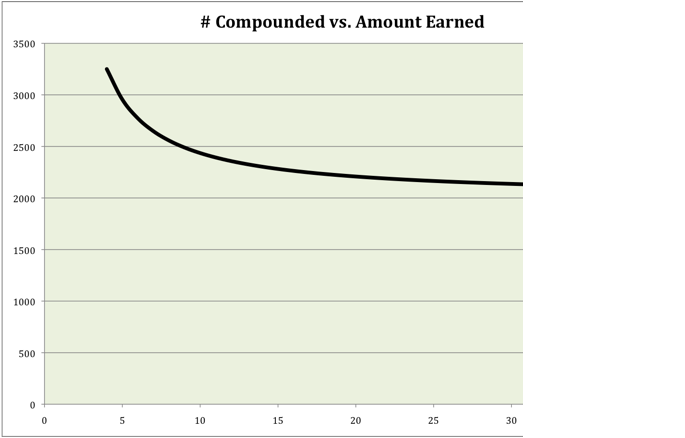
The
regression equation for this function is  . Again, if we plug our compounded value in for “x”, the
output will be the amount earned based on a $2,000 principal, 1.99% interest
rate and a 10 year period.
. Again, if we plug our compounded value in for “x”, the
output will be the amount earned based on a $2,000 principal, 1.99% interest
rate and a 10 year period.
We
can also find a function for the amount of time our money is in the bank. Let’s
look at the chart where the “year” variable changes.
|
Principal |
Interest
Rate (Annual) |
#of
Times Interest is Compounded per Year |
#
of Years |
Total
Amount in Account After N Years |
|
|
P |
r |
q |
n |
A |
|
|
2000 |
0.199 |
4 |
10 |
3250.04 |
|
|
2000 |
0.199 |
4 |
11 |
3328.28 |
|
|
2000 |
0.199 |
4 |
12 |
3408.20 |
|
|
2000 |
0.199 |
4 |
13 |
3489.85 |
|
|
2000 |
0.199 |
4 |
14 |
3573.26 |
|
|
2000 |
0.199 |
4 |
15 |
3658.45 |
|
|
2000 |
0.199 |
4 |
16 |
3745.47 |
|
|
2000 |
0.199 |
4 |
17 |
3834.35 |
|
|
2000 |
0.199 |
4 |
18 |
3925.12 |
|
|
2000 |
0.199 |
4 |
19 |
4017.82 |
|
|
2000 |
0.199 |
4 |
20 |
4112.49 |
|
|
2000 |
0.199 |
4 |
21 |
4209.16 |
|
|
2000 |
0.199 |
4 |
22 |
4307.87 |
|
|
2000 |
0.199 |
4 |
23 |
4408.65 |
|
|
2000 |
0.199 |
4 |
24 |
4511.56 |
|
|
2000 |
0.199 |
4 |
25 |
4616.62 |
|
|
2000 |
0.199 |
4 |
26 |
4723.88 |
|
|
2000 |
0.199 |
4 |
27 |
4833.38 |
|
|
2000 |
0.199 |
4 |
28 |
4945.15 |
|
|
2000 |
0.199 |
4 |
29 |
5059.25 |
|
|
2000 |
0.199 |
4 |
30 |
5175.71 |
|
|
2000 |
0.199 |
4 |
31 |
5294.57 |
|
|
2000 |
0.199 |
4 |
32 |
5415.89 |
|
|
2000 |
0.199 |
4 |
33 |
5539.71 |
|
|
2000 |
0.199 |
4 |
34 |
5666.06 |
|
|
2000 |
0.199 |
4 |
35 |
5795.01 |
|
|
2000 |
0.199 |
4 |
36 |
5926.59 |
|
|
2000 |
0.199 |
4 |
37 |
6060.85 |
|
|
2000 |
0.199 |
4 |
38 |
6197.84 |
|
|
2000 |
0.199 |
4 |
39 |
6337.62 |
|
|
2000 |
0.199 |
4 |
40 |
6480.22 |
|
|
2000 |
0.199 |
4 |
41 |
6625.71 |
|
|
2000 |
0.199 |
4 |
42 |
6774.13 |
Above,
we can see the effect that “number of years” has on the amount earned. Below is a graph of the data including
the regression equation and correlation coefficient.
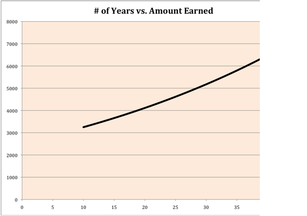
Again,
this equation is the natural log function  .
.
From
the above equations for principal, interest, number of times compounded, and
number of years in the account, we can estimate the amount earned based on any
one of these variables.