
Polar Equations
by Michael Walliser
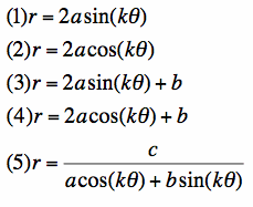
In this lesson, we will familiarize ourselves with polar equations where r is a function of theta. The periodic nature of trigonometric functions makes them interesting to view in polar coordinates, because they form "closed" shapes as they repeat themselves. We will look at a series of trigonometric polar equations and account for the changes in the graphs as we adjust the variables. The equations are listed below, and will be referred to as (1), (2), (3), (4), and (5).
Below is a graph of (1) with a = 1, and k values of 2 and 4.

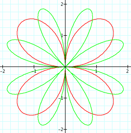
For each k value, we get a rose with 2k leaves. Let's trace the functions. When k = 2, we start at radius zero for theta = 0. Any coordinate for which r = 0 corresponds to the origin. When theta reaches 45 degrees, the argument of the sine function is 90 degrees, so the sine function reaches a maximum of 1. Since there is a coefficient of 2 (= 2a), this maximum radius is 2. The radius then descends, reaching zero at theta = 90 degrees, since the argument of the sine function is then 180 degrees. Thus we have traced the leaf in quadrant I. As theta moves into the second quadrant, the argument of the sine function moves into the third quadrant, so the function becomes negative. Therefore, since theta is in the second quadrant, the negative radius traces a leaf in the opposite direction, in the fourth quadrant. The minimum radius of -1 is reached when the argument is 270 degrees (theta = 135 degrees). This corresponds to the tip of the leaf in quadrant IV. Again, due to the 2a coefficient, the radius here is 2. When theta reaches 180 degrees, the argument is back to 0 (aka 360 degrees). As theta moves through the third quadrant, the argument repeats itself through quadrants I and II. Thus the radius is positive in the direction of quadrant III, resulting in that leaf. Finally, with theta in the fourth quadrant, the argument is negative, so the leaf is traced in the opposite direction, i.e. quadrant II. These values repeat themselves as theta continues around the circle, so we are left with a 4-leaf rose.
When k = 4, the leaves are traced in a similar manner, but the argument changes twice as fast with respect to theta. Therefore, a leaf is created for every 45 degree rotation of theta, resulting in 8 leaves before theta reaches 360 degrees and repeats itself. Note that each new leaf alternates whether the radius is in the positive or negative direction, so of the two leaves in each quadrant, one is from when theta is in that quadrant, and one is from when theta is in the opposite quadrant. Also, since the absolute value of the sine function goes in 180 degree cycles, one leaf is traced for every 180-degree increment of the argument.
Below is a graph of (1) with a = 1, and k values of 1 and 3.

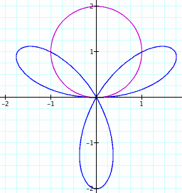
This time, for each k value, we get a rose with k leaves, if we count this circle as a "one-leaf rose". Let's trace the functions and figure out why. When k = 1, the graph starts out with theta = 0 and r = 0. When theta reaches 45 degrees, the argument becomes half the square root of 2. Since there is a coefficient of 2 (= 2a), the radius becomes the square root of two, hence the inclusion of the point (1,1). When theta reaches 90 degrees, the argument hits a maximum of 1, and because of the coefficient, the radius reaches 2. As theta moves through quadrant II, r follows the reverse path of quadrant I, thus the symmetry. When theta moves through quadrants III and IV, the sine function becomes negative, but with the same pattern of magnitude as in the first two quadrants. Therefore, the function traces a leaf in the same quadrants as the one it just traced. As such, we are left with a one-leaf rose for k = 1.
When k = 3, the function traces a leaf every 60 degrees that theta rotates (180/3 = 60). For theta from 0 to 60 degrees, the argument ranges from 0 to 180 degrees, so the sine function is positive, creating the leaf in the first quadrant. For theta between 60 and 120 degrees, the argument ranges from 180 to 360 degrees, so the sine function is negative, creating the leaf in quadrants III and IV. For theta between 120 and 180, the argument ranges from 360 (0) to 540 (180), so the sine function is positive, creating the leaf in the second quadrant. For theta from 180 to 240, the argument ranges from 540 (180) to 720 (0), so the sine function is negative, thus retracing the first leaf. For theta from 240 to 300, the argument ranges from 720 (0) to 900 (180), so the sine function is positive, and the graph retraces the second leaf. Similarly, the last range of theta retraces the third leaf.
We see that when k is odd, the function repeats itself once theta = 180 degrees. Therefore, we get a rose with k leaves as opposed to 2k leaves.
So we know what happens when k is even and when k is odd, but what about when k is not an integer? We'll let k = 3/2.
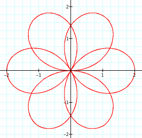
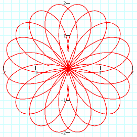
What happens is that now when theta gets back to 360 degrees, the function does not repeat itself. Whole number coefficients of theta simply transformed the argument into another version of 360 degrees. With a fractional coefficient, theta must make the 360 cycle a number of times (equal to the denominator) before it begins to repeat. This also causes an overlap in the leaves, resulting in a number of "levels" of leaves equal to the denominator (here we have the pointed, football-shaped leaves in the middle, and the larger, round leaves on the outside). If our coefficient is the reduced fraction a/b, then there are 2a "major" leaves and b "levels" of leaves. Another example is shown below, where k = 9/4.
Now let's fix k = 3 and see what happens when we use different values of a.
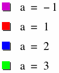
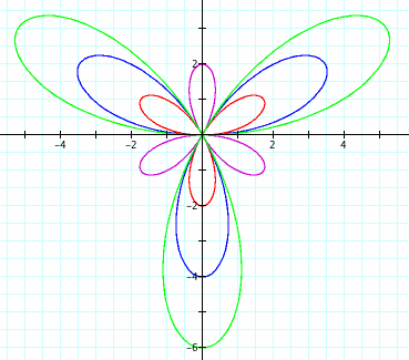
It shouldn't be surprising that, since a is a coefficient of the entire function, adjusting a simply changes the magnitude. We also see that a negative value of a flips the graph upside down. Because there is a coefficient of 2a on the sine function, the maximum radius reached on each of these graphs is 2a.
Since the sine and cosine functions are similar, we expect the graphs from equation (2) to resemble those from equation (1) above. We'll again start by fixing a = 1, and looking at k values of 2 and 4.

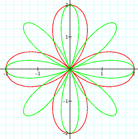
We again see the roses with 2k leaves, but they are oriented slightly different this time. Since the cosine function is equal to 1 at theta = 0, the tip of the first leaf is located on the positive x-axis. In tracing this function (k = 2), the first leaf starts at the tip, and is traced halfway (in quadrant I), then the second leaf is traced with the tip on the negative y-axis, then the third leaf on the negative x-axis, the fourth on the positive y-axis, and finally the first leaf is finished as theta reaches 360 degrees.
Below are graphs of (2) with odd values of k.

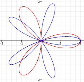
As expected, we have roses with k leaves, oriented so that the tip of the first leaf is on the positive x-axis.
If we were to adjust the value of a we would again see a change in magnitude, and if we were to use a fractional value of k, we would again see roses with multiple levels of leaves.
Let's move on to equations (3) and (4). We'll start with equation (3) and fix a = 1 and k = 2, while varying b. First, let's see what happens when b increases from 0 to 3.
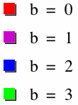
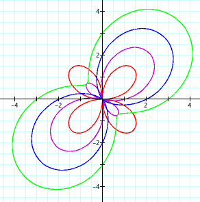
Obviously, when b = 0, we have a replica of our graph from above. Recall that the leaves in quadrants I and III were created when r > 0 and the leaves in quadrants II and IV were created when r < 0. We know that because a = 1, the term 2asin(k*theta) has limits of -2 and 2. Adding a constant to this term shifts the limits up or down. When b = 1, the limits of r are -1 and 3. As the positive range grows, the size of the "positive" leaves grows. Likewise, as the negative range shrinks, so does the size of the "negative" leaves. When b = 2 (or more generally, when b = 2a), the negative range disappears, as do the "negative" leaves. Once b is greater than 2a, there is no longer a value of theta that will make r equal to zero, so the graph no longer crosses the origin.
When we decrease b from 0 to -3, we see the opposite happen. The "positive" leaves shrink and then disappear, and once b < 2a, the value of r never climbs back up to 0, so the graph no longer crosses the origin, as shown in the graph below.
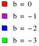
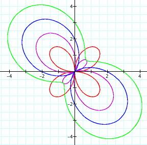
Note that if we change the value of a, the magnitude of the graphs will change, and the critical value of b at which one pair of leaves disappears will always the +/- 2a, the coefficient of the sine function.
Recall in equation (1) that when k is odd, after theta reaches 180 degrees, "negative" leaves begin to trace directly on top of "positive" leaves. So can you guess what happens to such a function when we throw the variable b into the mix?
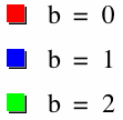
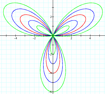
In this graph, a = 2 and k = 3. We see that, just as when k is even, the "positive" leaves grow as the "negative" leaves shrink. This time, however, the positives and the negatives lie on the same lines. Consequently, if b were negative, we would see the exact same results. Just for the sake of visualization, the graph below shows the graph as b becomes greater than 2a.
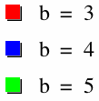
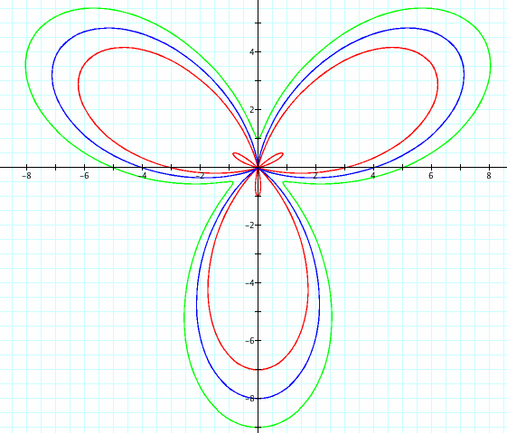
We again see the graph "let go" of the origin once b > 2a.
Since the principles behind the cosine function in equation (4) are so similar to those of the sine function, we really don't need to analyze it too deeply. Just as equation (2) produced the same traits on its graphs as equation (1) with a different orientation, so too does equation (4) mirror equation (3). Below is the example with a = 1 and k = 2.

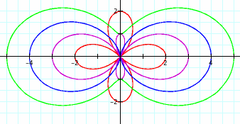
As expected, we see the "negative" leaves shrink and disappear, and then when b > 2a, the graph no longer passes through the origin.
Before we look at equation (5), let's look at the function in the denominator. As we change k, we see that the number of leaves still holds to our rule of k for odd values, and 2k for even values. In the graph below, a = 3 and b = 3.
![]()

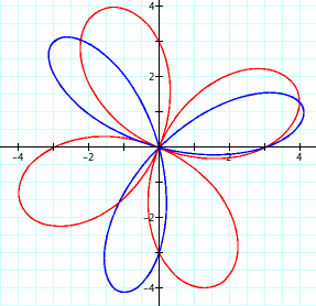
Notice that the orientation of these graphs is somewhere between those of the sine and cosine functions by themselves. Changing a and b independently will change the magnitude, and as one gets drastically larger than the other, the graph is "pulled" in the direction of that variable's function (cosine for a, sine for b). The graph below shows an example with k = 2.
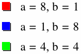
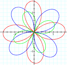
We can see that the red curve is oriented almost the same as the cosine function, while the blue curve is oriented almost the same as the sine function. Both are larger in magnitude than the green curve.
Now that we have a bit of an understanding about that function, we can look at equation (5), which is simply its inverse. We should expect the radius to approach infinity at the same places the curves above would approach the origin, and the radius should reach a minimum in the same place that we see the tips of the leaves above. Below on the left is a graph of equation (5), with a = 1, b = 1, c = 10, and k = 2. The straight lines drawn in are asymptotes and are not part of the curve. On the right is its inverse. Note that the graphs are not on the same scale.
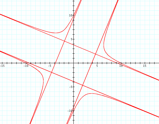
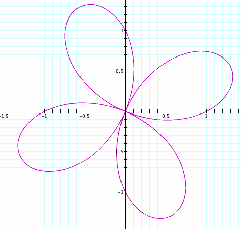
Indeed, the curve has minima where we expect and approaches infinity where we expect. We should also expect that since c is a coefficient to the entire term, it should directly influence the magnitude of the curve. Let's see, with k = 5, a = 1, and b = 1.
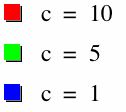
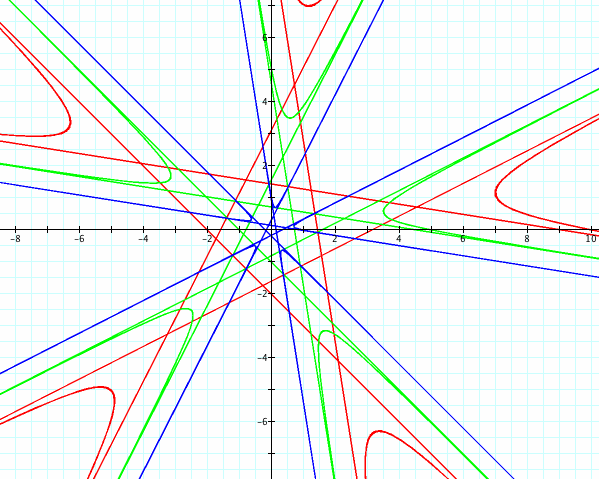
Try to ignore the asymptotes and you will see that yes, as c decreases, the curve comes closer to the origin. Also note that since k = 5, there are 5 branches to each curve. It is easy to see that this function follows the properties predicted by its inverse. As a final observation, we will look at the curve when a >> b and when b >> a, with c = 10 and k = 2.

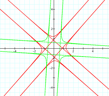
As we saw before, when the coefficient a of the cosine term was much larger than the coefficient b of the sine term, the function was "pulled" toward the cosine function, which had the tip of its first leaf located on the x-axis. Here, in the inverse function, we see that a minimum occurs near the x-axis when a >> b, but when b >> a, the minimum occurs near the 45 degree mark, where the tip of the leaf is on the sine function (when k = 2).