

Assignment III: Parameters of Quadratic Equations
by
Rui Kang
Investigation 1.
It has now become a rather standard exercise, with available technology, to construct graphs to consider the equation
![]()
and to overlay several graphs of
![]()
for different values of a, b, or c as the other two are held constant.
From these graphs discussion of the patterns for the roots of
![]()
can be followed.
The next graph demonstrates happens if we hold b and c constant, in particular, b=c=1 and vary the value of parameter a:
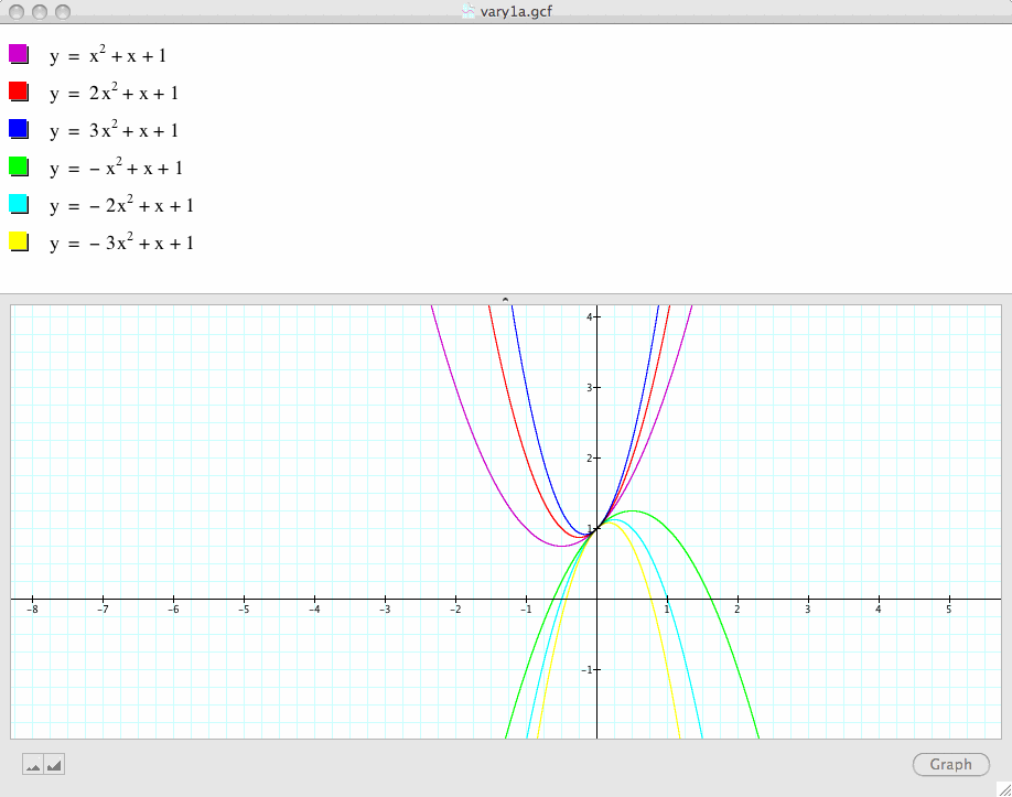
Observe the above graph, we note that this family of parabolas always passes through the point (0,1), which is understandable because when x=0,
substitute x into the quadratic equation, we get y=1;
thus (0,1) is always a solution to this family of parabolas even if we let a take other values such as -4, 5, 37, -104 etc.
Conclusion 1: From this observation, we can generalize that if we change the value of a, for positive a, we get a family of parabolas opening up;
for negative a, we get a family of parabolas opening down; and finally, but all these parabolas pass through a common point, i.e., (0, c).
(A side note is that when a=0, the graph is not a parabola anymore because it violates one of the conditions of a quadratic equation.
Under this particular case when a=0, the graph is a line y=1, but note that the graph still passes through the point, (0,1).)
The next couple of graphs examine what happens if we vary the parameter b, while holding a and c constant. For example, if we set
![]()
and let b takes values -3, -2, -1, 0, 1, 2, 3, and overlay the graphs, the following picture is obtained:
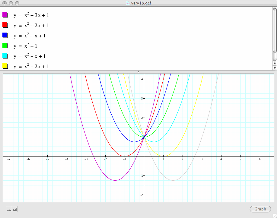
We can now discuss the "movement" of a parabola as b changes. The parabola always passes through the same point, (0, C), on the y-axis (the point (0,1) with this equation).
Next, let's consider the locus of the vertices of this family of parabolas graphed from
![]()
In particular, we want to show that the locus is a parabola.
Use the "completing square" method to rewrite the above equation,
we get

Factoring, and replacing b by n for purposes of animating a graph we have

This suggests that the vertex is at
![]()
If we name this vertex point as (d, f), then d and f satisfy
d=![]() , f=
, f=  ,
,
substitute d to the f equation, we have f=![]() , or a parabola.
, or a parabola.
We have shown without using calculus that the locus of the vertices of the set of parabolas graphed from
![]()
is indeed a parabola.
The following graph further illustrated this fact:
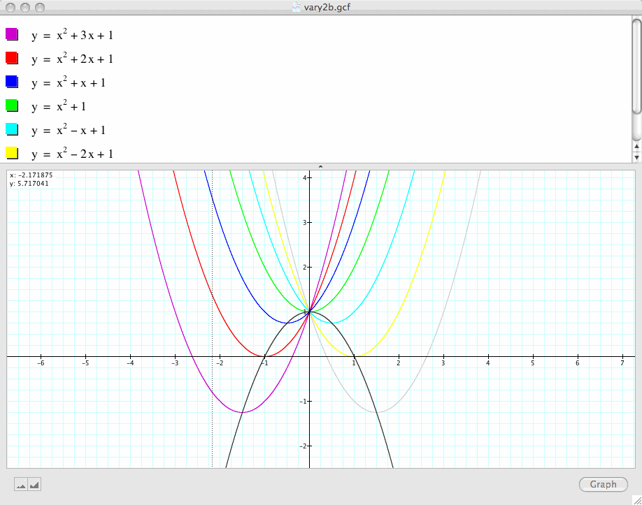
Conclusion 2: As b changes, the parabolas still pass through the same point, (0, C), on the y-axis (the point (0,1) with this equation).
When the parabola intersects the x-axis at two point, the quadratic equation has two roots.
When the parabola is tangent to the x-axis, the quadratic equation has one root.
When the parabola does not intersect the x-axis at all, the quadratic equation has no roots. In addition, the locus of the vertices of the set of parabolas is yet another parabola.
In the next graph, we explore what happens if we hold a and b constant and vary the values of c:
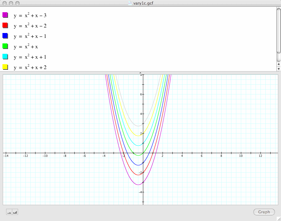
Conclusion 3: As c changes, the parabola moves up and down, but remains the same shape with one nesting within another.
Investigation 2.
Consider again the equation
![]() ,
,
but this time, instead of graphing it in our standard coordinate system, we graph this relation in the xb plane.
If we take any particular value of b, say b=5, and overlay this equation on the graph, we add a line parallel to the x-axis.
If the line intersects the curve in the xb plane, the intersection points correspond to the roots of the original equation for that value of b. We have the following graph:
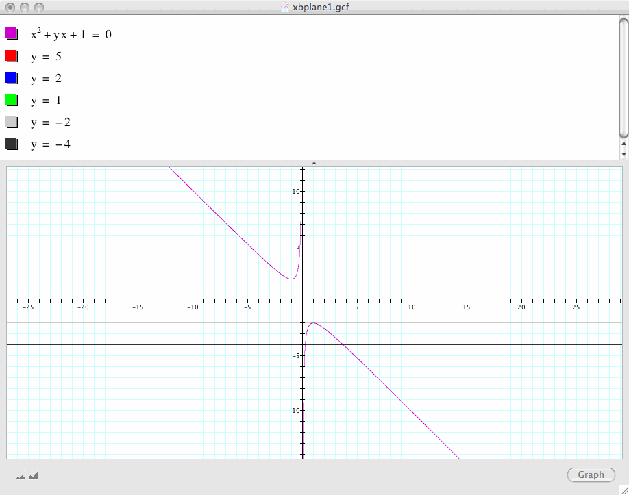
For each value of b we select, we get a horizontal line.
It is clear on a single graph, that we get two negative real roots of the original equation when b>2 (observe the red line, b=5),
one negative real root when b=2 (observe the blue line, b=2),
no real roots for -2<b<2 (observe the green line, b=1),
one positive real root when b=-2 (observe the grey line, b=-2),
and two positive real roots when b<-2 (observe the black line, b=-4).
Now let's try different values of c instead of c=+1:
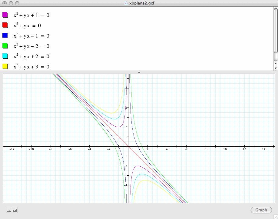
First, we observe that as we vary the value c, we get a set of nested curves.
Second, a particular value of c, i.e., c=0 catches our attention. This curve corresponds to the equation:
![]()
If we factor this equation, we have x(x+y)=0. This suggests that we get two lines: x=0 (i.e., the y-axis) and y=-x (the red line in our graph)
If we observe the relation between these two lines and the set of curves, we find that these two lines in fact are the two asymptotes of the parabolas.
Third, we may again take any particular value of b, say b=5 and overlay this equation on the graph, then we add a line parallel to the x-axis.
If the line intersects the curve in the xb plane, the intersection points correspond to the roots of the original equation for this value of b.
Interestingly, we observe that when c is negative (look at the blue or green line), the equation always has two roots, one positive and one negative.
This is because we know that for any quadratic equation, when ![]() , it has two real roots; when
, it has two real roots; when ![]() , it has one real root;
, it has one real root;
when ![]() , it has no real roots.
, it has no real roots.
So for
![]() ,
,
it always has two real roots when
![]() .
.
But when c<0, the above inequality is always true. This is the reason that we observe that when c is negative, the equation always has two roots.
For positive values of c, on the other hand, we need to use the same method earlier by letting b take on different values
and observe when the horizontal line intersects the curve at two points (two roots), one point (one root), or no point (no root).
And we may call this method, "the horizontal test".
Investigation 3:
Now let's add the graph of 2x+b=0 to the picture and discuss its relation to the quadratic formula:
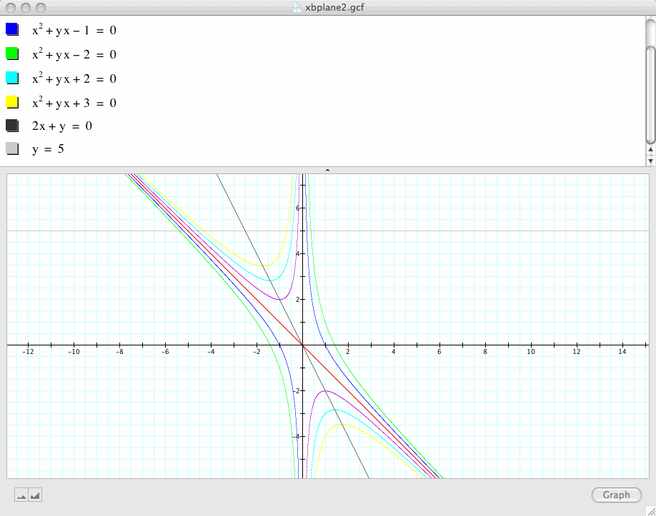
Clearly, this line passes through all of the vertices of the set of parabolas when c>0.
A little calculus can help us explain why this is the case.
Observe the set of quadratic equations in the graph, and we see that 2x+y=0 is the first derivative of each one of the functions graphed.
We further observe that when c>0, the curves/parabolas change directions when they cross the line, 2x+y=0.
And by the first derivative test, this is exactly where the relative maximum or minimum occurs.
(A side note is that: for c<0 or c=0, the curves do not have a relative maximum and minimum. And the line 2x+y=0 does not pass those curves.)
Investigation 4:
So far we have only graphed the quadratic equation in the xb plane, you may ask what happens if the graphs are in the xc plane or xa plane.
In this particular investigation, we look at the case for the xc plane. In Investigation 5, we look at the case for the xa plane.
In particular, in the next graph, we allow b to vary from -3, -2, -1, 0, to 1, 2, and 3 and observe what happens:
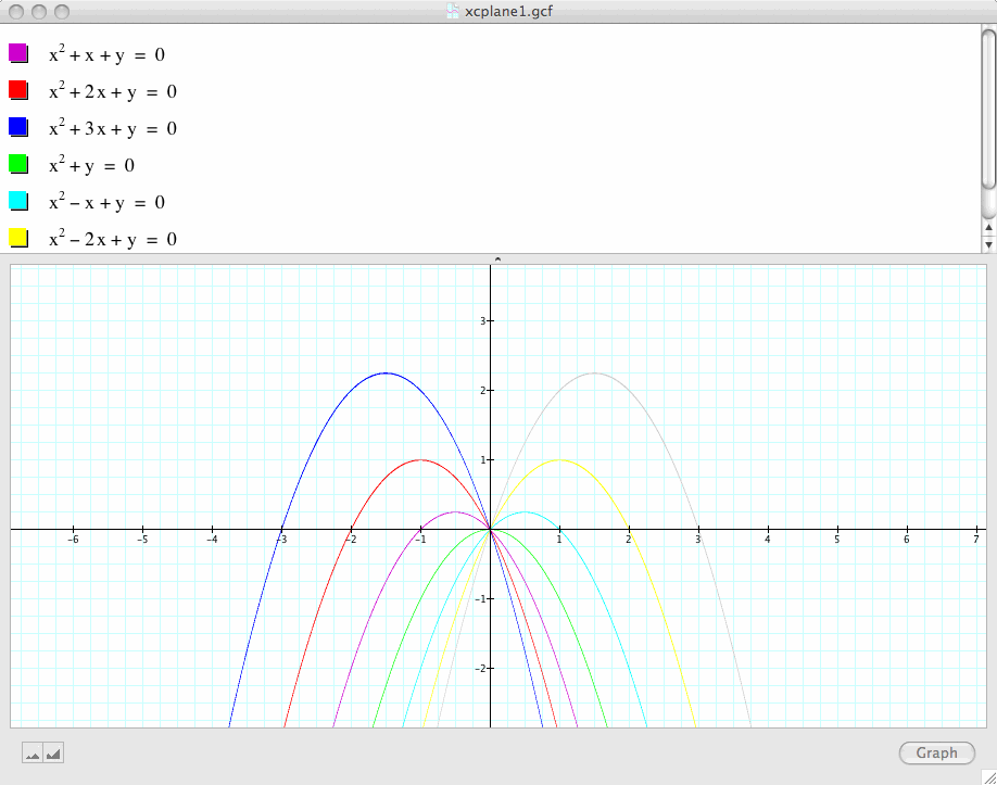
In this case, we observe that all of the parabolas pass through the origin (0, 0), which is understandable
because when x=0, y=0, i.e., (0, 0) is always a common root for this set of the equations.
Another rather interesting observation we could obtain from this set of graphs is that the y-coordinate of the vertices of this set of parabolas have particular relations to
whether the quadratic equation has solutions and how many solutions it has. This will seem much easier if we look at an example:
Observe the yellow curve
![]() ,
,
its vertex is at (1,1) whose y-coordinate is 1.
If we use our knowledge in algebra, we know this quadratic equation will have a real solution if
![]() , i.e.,
, i.e., ![]() , or
, or ![]() for b=-2. In particular, the quadratic equation will have two real roots if y<1,
for b=-2. In particular, the quadratic equation will have two real roots if y<1,
and precisely one real root if y=1, and no real solution if y>1.
Therefore, by observing where the vertex of a parabola is located in the xc plane,
we can derive what values c should take in order for the corresponding quadratic equation to have two real roots, one real root, or no real roots.
Try this with any of the other curves in the above picture and see whether the above observation applies to all of them!
Investigation 5:
Finally, let's observe what happens if our graphs are in the xa plane. In particular, let's vary c from -3, -2, -1, 0, 1, 2, and 3:
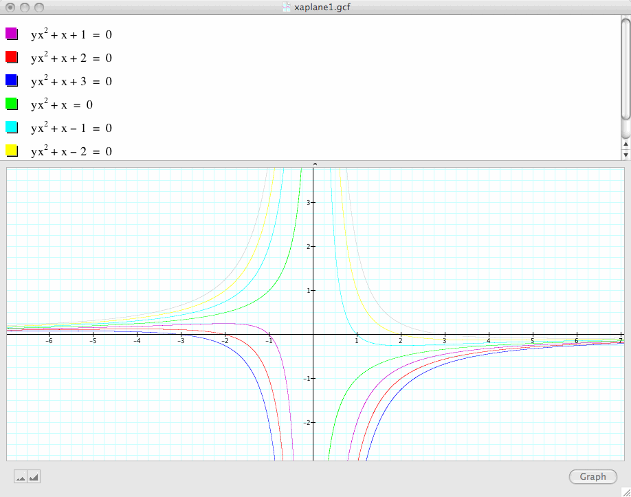
In fact, this graph does not give us as much information as those in the xb and xc plane.
We may observe, though, that as c=0 the graph of
![]()
never crosses the x-axis (in green), whereas the rest of the graphs all have half of them cross the x-axis.
For c>0, as x approaches 0, y approaches negative infinity; for c<0, as x approaches 0, y approaches positive infinity.
A closer examination of the quadratic equation, we find that ,
![]()
unlike the rest of the equations, always have real solutions because when x=0, y can take on any value.
But for the rest of the equations, for some y values, the equation have two real roots or one real root; whereas for other y values, the equation may not have real roots.
We have finally reached the end of this long investigation.
Hopefully this write-up gives you more insights about the relations between the properties of a quadratic equation and how its graph looks like.