

In this brief exploration, we will explore the following equation for different values of parameters 'a' and 'b'. We will investigate the shape of the graph for different values of 'a' and 'b,' and look for relationships between them. The exploration will be conducted using a graphing program.
![]()
How does this function look like? Let us begin the exploration by taking a look into a simple case of the equation, when a = 4 and b = 1. The graph looks like the following.
![]()
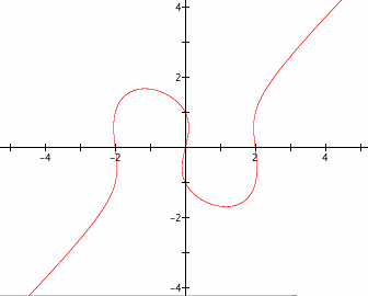
The graph is interesting (well kind of), it looks similar to a general third order function of x with the curves being cooler. The graph crosses the x-axis at x = -2, 0, 2, and crosses the y-axis at y = -1, 1, as expected from the equation above.
Let us see how changing the parameter 'a' affects the shape of the graph. We will do this by starting with the simple case when a = 4 and b = 1, and then graph the equation for different ranges of values of 'a'.
i) 'a' above 4
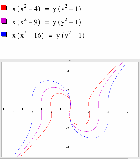
As the value of 'a' increases above a = 4, the size of the loop increases both vertically and horizontally. Note again where the graph crosses the x-axis and the y-axis.
The roots of the graph can be found by setting y = 0 which gives
![]()
and solving the equation, which gives
![]()
ii) 'a' decreases from a = 4 to a = 1
Now what happens if we make the parameter 'a' decrease from a = 4 to a = 1?
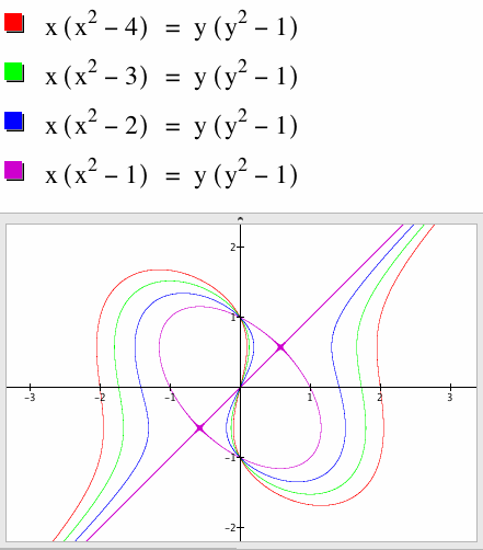
The pattern is as expected until we get to a = 1, and then suddenly something strange and out of ordinary happens. Why is this so?
Consider the equation when a = 1. The equation is
![]()
We can rearrange the equation as,
![]()
and use a factoring equation to get

where the last line is the equations of a straight line and an elipse respectively.
iii) 'a' is smaller than 1
Now, let's look at when 'a' is smaller than 1.
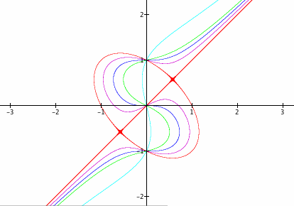
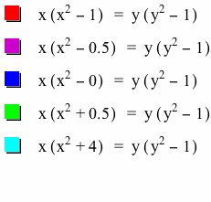
We can see that, for a < 1, the directions of the loops have changed, but is the same shape. With 'a' getting smaller, the size of the loop also gets smaller.
Let's now look at how the parameter 'b' affects the graph. We will hold 'a' constant at a = 1, and increase the values of b, and take a look at the graph.
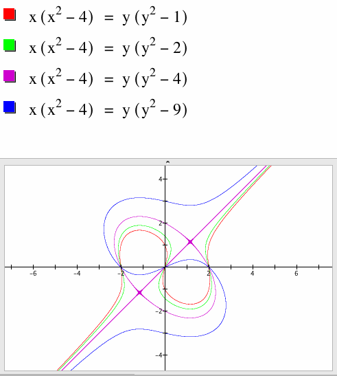
Increasing the values of 'b' increases the size of the loop, until b < 4, and then at b = 4 (purple), we again have the ellipse plus straight line shape. When b > 4, the direction of the loop changes, and the size of the loop increases as b increases above b = 4.
Therefore, there seems to be a special relationship between the relative size of the two parameters 'a' and 'b'. Note that at a = b, we obtain the special case of ellipse plus the line, which can be proved by the same factoring equations that was used above. And the direction of the opening of the graph depends on whether a > b or a < b.
Thus, we conclude that the parameters are interelated, and it is the relative size of 'a' and 'b' that determines the general shape of the graph. The general shape of our main equation
![]()
looks like the following:
When a > b,
|
When a = b,
|
When a < b
|
Let's say we want to construct a graph that looks like the following:
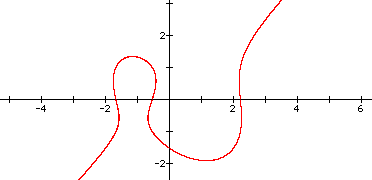
How do we construct such a graph?
This graph has a similar shape from the graphs in the first investigation, but differs in the size of the loops. Specifically, the size of the loops are not symmetric any more.
One approach is to observe the roots on the x-axis from the graph in question and adjust the main equation from the first investigation. We will start with the same intial equation from the first investigation,
![]()
and play around with it.
Since the roots in the above graph seem to go through the x-axis at x = -1.7, -0.7, and 2.2, let's contstruct an equation such as
![]()
and graph it.
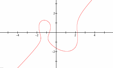
Sweet! The graph is very close to the one in question.
What are some other ways to reach a similar graph? It will be left as an exercise for further explorations. Possibly, there is a relation between the numbers 1.7, 0.7, 2.2 with some combinations of square root of integers, that enables a simpler equation.
In this exploration, let us add a constant to the main equation and investigate the shapes of the graphs. Let us set up the equation as
![]()
and see how adding a constant affects the function.
We can animate the above function for various values of z, and see the graph. In the animation below, I chose z to range from -10 to 10.
By pausing the animation, we can see the graph that was wanted from the "Further Exploration" section. The value of z is approximately 1.8 when this happens.
Now, back to this exploration, by trial and error, I found that the graph separates into two sections around z = -2.7, 2.7 and the circle section disappears around z = -3.5, 3.5.
What happens around these values of z? It is likely related to how many roots the function of x on the left has at different ranges of values. This search for explanation will be left for another time.