

The quadratic function of x is a second order function of x that is generally expressed as ![]() , where a, b, and c are constants. The graph of the quadratic function is a parabola that looks like a U shaped curve. The quadratic function is well-known, and the basic properties of a quadratic function can be found in many websites and textbooks.
, where a, b, and c are constants. The graph of the quadratic function is a parabola that looks like a U shaped curve. The quadratic function is well-known, and the basic properties of a quadratic function can be found in many websites and textbooks.
In this investigation, we will explore how adding a xy term the quadratic function ![]() affects the shape of the graph. The general equation under exploration will be
affects the shape of the graph. The general equation under exploration will be ![]() .
.
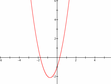
Let us begin with the quadratic function ![]() which looks like the following graph.
which looks like the following graph.
Now, let's add the xy-term to the right side of the above equation, so that we get ![]() , and graph it.
, and graph it.
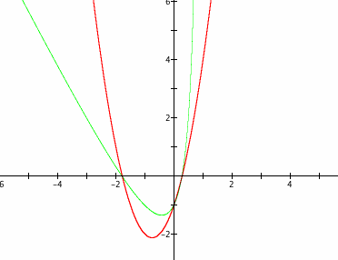
The effect of the xy-term seems easy to explain at first. However, could there be another part of the new graph (green) missing? When x = 2, solving the equation![]() for y gives y = -13, so we are likely missing a part of the graph somewhere in the fourth quadrant. Zooming out of the graph reveals that there is a secret hidden part of the new graph.
for y gives y = -13, so we are likely missing a part of the graph somewhere in the fourth quadrant. Zooming out of the graph reveals that there is a secret hidden part of the new graph.
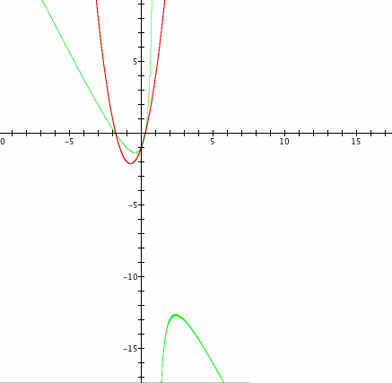
Now lets take a careful look at the new graph with the xy-term and observe any patterns. The quadratic with the xy-term has two separate parts, and each of them looks like a tilted quadratic. The upper-left part of the new graph have three common points with the original quadratic, and the three common points are the x and y-intercepts of the original quadratic. What else did you notice?
It is interesting and important to note that there seems to be an asymptote at x = 1. In fact there is an asymptote, and the equation of the asymptote can be found by solving for y in terms of x in the new equation. Solving for y in terms of x gives,
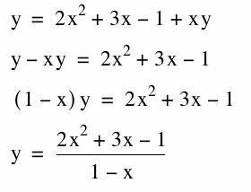
Since 1 - x cannot equal to zero (a number cannot be divided by zero), we see that the equation of the asymptote is x = 1.
We will start investigating the affect of the xy-term, by graphing the equation ![]() for various values of m and comparing the shapes of the graphs. First let us observe the graph for positive values of the coefficient m.
for various values of m and comparing the shapes of the graphs. First let us observe the graph for positive values of the coefficient m.
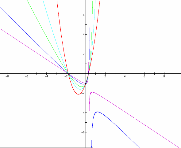
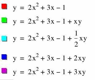
Some observations:
1. As the coefficient m of the xy-term increases, the graph continues to open up more and more. (The graph becomes more wide.)
2. As the coeffient m approaches zero, the upper-left part of the graph draws closer to the original quadratic equation without the xy-term (red), while the lower-right graph separates further away from the upper left graph. Clearly, as the coefficient m approaches 0, the quadratic equation with the xy-term approaches becoming the original quadratic equation.
3. Interestingly, all the upper-left part of the graphs with the xy-term crosses through the same three points which are on the x-axis and the y-axis. Why is this so?
This is because all the graphs in the form ![]() has the same x- and y-intercepts as the original quadratic equation, because the addition of the mxy-term does not affect the x- and y-intercept values. This becomes more clear when we solve for the x- and y-intercepts of
has the same x- and y-intercepts as the original quadratic equation, because the addition of the mxy-term does not affect the x- and y-intercept values. This becomes more clear when we solve for the x- and y-intercepts of ![]() . Remember that when we solve for the x- or y-intercepts, we need to set x = 0 or y = 0, and setting either x = 0 or y = 0 will make the mxy-term equal to zero so that the mxy-term has no effect on the x- and y-intercept values.
. Remember that when we solve for the x- or y-intercepts, we need to set x = 0 or y = 0, and setting either x = 0 or y = 0 will make the mxy-term equal to zero so that the mxy-term has no effect on the x- and y-intercept values.
4. The vertical asymptote draws closer to the y-axis as the coefficient m is increased. This can be explained by solving for the equation of the asymptote, in the same manner in the above section.
Now lets observe the graphs when the coefficient m of the equation ![]() is negative. The red-colored graph is the original graph without the xy-term, and the graph for m = -0.5, m = -1, and m = -2 is shown in the following graph. (as color green, blue, and purple)
is negative. The red-colored graph is the original graph without the xy-term, and the graph for m = -0.5, m = -1, and m = -2 is shown in the following graph. (as color green, blue, and purple)
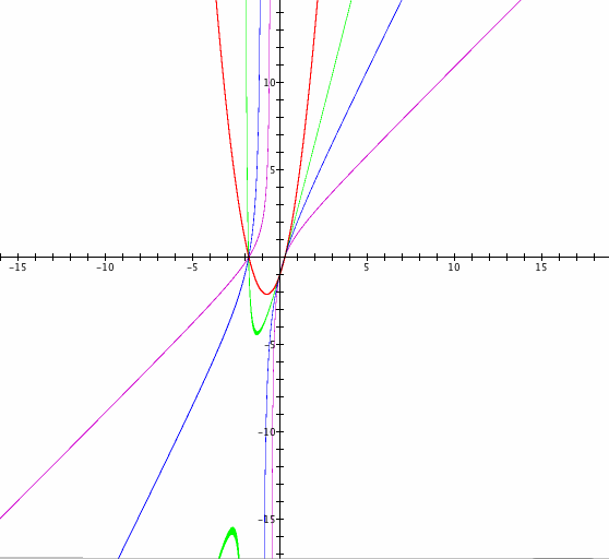
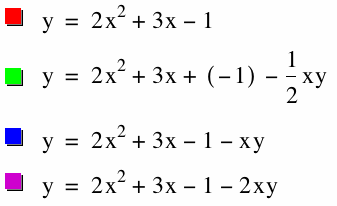
At first, when a = -1/2, the graph tilted to the right, and the usual pattern from m > 0 seemed to continue. However, when we set a = - 1 and a = - 2, we suddenly obtain graphs with new shapes of hyperbolas. Hence, there is a change in the shape of the graphs for different values of m.
Let us explore this transition point from one shape of hyperbolas to another. We know that the transition happens somewhere between a = - 1 and a = - 0.5. Let us look into the graphs in the range - 1 < a < - 0.5 and zoom in to get an approximation of the transition timing.
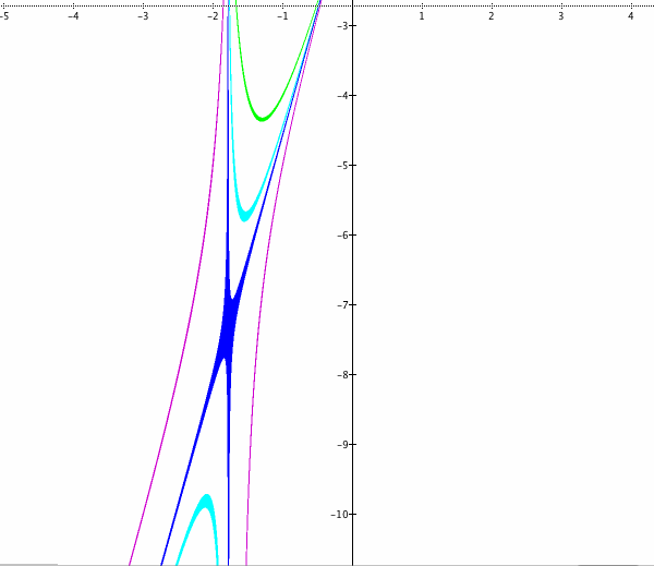
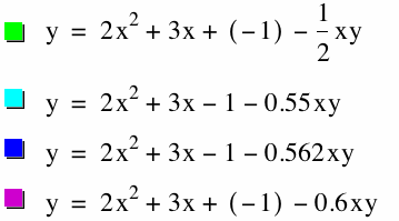
The transition occurs at approximately m = - 0.562, and the coordiantes of the point of separation is approximately ( -1.8, -7.0).
The investigation in the above section suggests that there might be another transition point for m > 0 which we did not notice in the first section. Let us graph![]() for larger values of m > 0.
for larger values of m > 0.
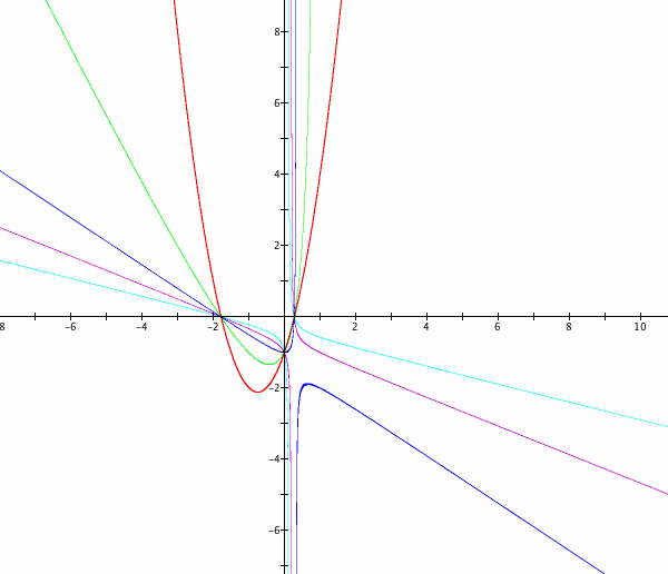
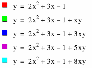
Another transition in the shape of the hyperbolas occurs between 3 < m < 5. The transition occurs at approximately m = 3.56, as can be seen from the graph below which is zoomed in.
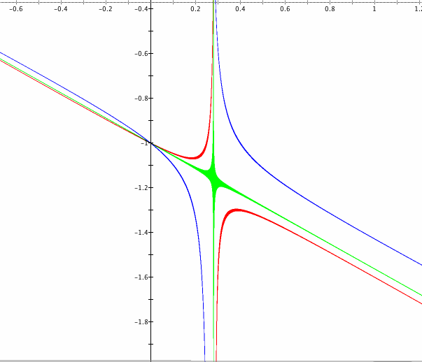
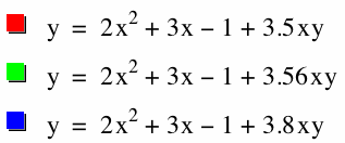
Why is there a change in the shape of the graph at m = - 0.562 and m = 3.56?
Let's consider again the equation ![]() and rewrite it as,
and rewrite it as,
![]()
The equations of the graph at which the transition occurs are,
 ,
, 
The transition point is most likely related to the coefficients of the original quadratic, and there is probably a relationship that can be found. However, this is beyond the scope my ability, and the explanation will be left as a further exploration.
For and equation in the form ![]() ,
,
- If m < - 0.562, the graph is two hyberbolas that opens in the direction of the second and fourth quadrant.
- If -0.562 <m< 0, then the graph is two parabolas that are tilted to the right.
- For 0 < m < 3.562, we get two parabolas that are tilted to the left.
- And finally, when m > 3.562, we get two hyperbolas that opens in the direction of the first and third quadrant.
An animation is included to demonstrate the conclusion. (The range of m is -5 <m < 5.)