
With available technology, it has now become possible to construct graphs to consider the equation
![]()
and to overlay several graphs of
![]()
for different values of a, b, or c as the other two are held constant. From these graphs discussion of the patterns for the roots of
![]()
can be followed.
For the quadratic
![]()
lets set b = -3, -2, -1, 0, 1, 2, 3, and overlay the graphs.
We can discuss the "movement" of a parabola as b is changed. Note that the parabola always passes through the same point on the y-axis ( the point (0,1) with this equation).
For b < - 2 the parabola will intersect the x-axis in two points with positive x values (i.e. the original equation will have two real roots, both positive). For b = - 2, the parabola is tangent to the x-axis and so the original equation has one real positive root at the point of tangency. For -2 < b < 2, the parabola does not intersect the x-axis -- the original equation has no real roots. Similarly for b = 2, the parabola is tangent to the x-axis (one real negative root) and for b > 2, the parabola intersects the x-axis twice to show two negative real roots for each b.
Now consider the locus of the vertices of the set of parabolas graphed from
![]()
As we can see from the picture above, the locus looks like a parabola. And in fact, the locus is a parabola.
One approach is to complete the square with the first two terms on the right side of the equation to get
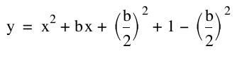
Factoring gives,
The above completion of the square is done to obtain the coordinates of the vertices. Remember that for a quadratic in the form ![]() , the coordinates of the vertices are (p, q).
, the coordinates of the vertices are (p, q).
Thus, the locus of the vertices of ![]() follow along the points (p, q) where
follow along the points (p, q) where
This set of equations can be solved as a function of p and q. First, solving for b in the first equation gives b = -2p, and substituting this into the second equation gives,
Hence, the equation of the locus of the vertices of ![]() is
is ![]() , as seen in the following graph.
, as seen in the following graph.
Consider again the equation
![]()
Now we will graph this relation in the xb plane. We get the following graph.
Note that the horizontal axis is still the "x"-axis, whereas the vertical axis is the "b"-axis in this case.
If we take any particular value of b, say b = 5, and overlay this equation on the graph, we add a line parallel to the x-axis. If it intersects the curve in the xb- plane the intersection points correspond to the roots of the original equation for that value of b. We have the following graph.
For each value of b we select, we get a horizontal line. It is clear on a single graph that we get two negative real roots of the original equation when b > 2, one negative real root when b = 2, no real roots for - 2 < b < 2, one positive real root when b = - 2, and two positive real roots when b < - 2.
Now lets consider a new equation ![]() . Note that we have a different value of parameter c in this case. As in the first part of the Investigation 2, graphing the equation in the xb plane gives
. Note that we have a different value of parameter c in this case. As in the first part of the Investigation 2, graphing the equation in the xb plane gives
Remember that if we set b to any value, say b = 3, and add this line to the graph, the intersection points correspond to the roots of the original equation for that value b. For every horizontal line that corresponds to a value of b, it is clear that every horizontal line intersects the graph at two points. This means that the original equation ![]() has two distinct real roots for every value of b.
has two distinct real roots for every value of b.
Also, since the graph in the xb-plane has two hyperbolas where one hyperbola is left of the y-axis and the other is right of the y-axis, the two roots of the original equation always has one that is positive and the other that is negative.
We see that depending upon the value of the parameter c, the quadratic equation ![]() have different ranges of value b that have two distinct real roots. Let us graph
have different ranges of value b that have two distinct real roots. Let us graph ![]() in the xb-plane for different values of c.
in the xb-plane for different values of c.
By observing the graph, a clear pattern emerges.
- For c > 0, the equation ![]() has different values of b that can give two roots, one root, or no root at all.
has different values of b that can give two roots, one root, or no root at all.
- For c = 0, the equation ![]() will always have two roots (one part of the light-blue graph lie along the y-axis), with one of of the roots always being x = 0.
will always have two roots (one part of the light-blue graph lie along the y-axis), with one of of the roots always being x = 0.
- For c < 0, the equation ![]() will always have two roots, one of them always being positive and the other always being negative.
will always have two roots, one of them always being positive and the other always being negative.
Let us add the graph 2x + b = 0 to the above graph of ![]() in Investigation 2.
in Investigation 2.
The graph 2x + b = 0 looks like it is going through the middle of each graph. This can be proved by taking the first derivative of
![]()
which gives
2x + b = 0
The graph 2x + b = 0 shows where the vertices of the equation ![]() are for each value of b. Since the two roots of a quadratic (if the quadratic has two real roots) are of equal distance from the vertex, the line 2x + b = 0 goes through the middle of each graph in the picture above.
are for each value of b. Since the two roots of a quadratic (if the quadratic has two real roots) are of equal distance from the vertex, the line 2x + b = 0 goes through the middle of each graph in the picture above.
Now lets consider graphs in the xc plane. We will start off with the equation
![]()
and graph it in the xc plane to get
Adding the graph of c = m, where m is any constant, will either intersect the original graph or not. If it intersects the curve in the xc-plane, then the intersection points correspond to the roots of the original equation for that value c.
If c > 1, then the original equation ![]() has no real roots, and if c = 1 the original equation has one root of x = - 1, and if c < 1 then the original equation has no real roots.
has no real roots, and if c = 1 the original equation has one root of x = - 1, and if c < 1 then the original equation has no real roots.
It is straighforward how the value of parameter c effects the roots of the equation of a general quadratic ![]() , since we know that a change in the value of c results in a vertical shift without any change in the shape.
, since we know that a change in the value of c results in a vertical shift without any change in the shape.
Let us look at the xa-plane of the following equation
![]()
by graphing the equation.
Similar to the investigations above, the line of a = m where m is any constant will show where the roots of the equation ![]() are. By looking at how the line a = m intersects the above graph, we can see that:
are. By looking at how the line a = m intersects the above graph, we can see that:
- for a > 1, the original equation has no real root,
- for a = 1, the orginal equation has one real root of x = - 1,
- for 0 < a <1, the original equation has two negative roots, of which one is always in the range -0.5 < x < -1, and the other approaching negative infinity as 'a' gets smaller,
- for a = 0, the original equation has one real root of x = -0.5
- for a < 0, the original equation has two roots, of which one is always in the range 0 < x < -0.5, and the other root always being positive.