
Assignment 10: Parametric Curves
Presented by: Amanda Oudi
Problem: Graph x =
cos(t) and y = sin(t). How would you change the equations to explore other
graphs?
Discussion:
I expect
that the graph of x = cos(t) and y = sin(t) for 0 < t < 2pi would form a
unit circle. From precalculus, I recall that on the unit circle that the
x-value corresponds to the trigonometric function cosine and the y-value
corresponds to the trigonometric function sine. Using Graphing Calculator 3.5,
let's check if my conjecture x = cos(t) and y = sin(t) for t between 0 and 2pi.
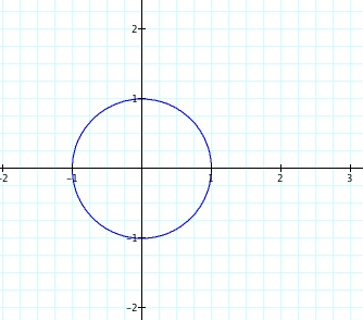
Looks as if my conjecture was correct! The reason a circle was produced is because t goes from 0 to 2pi. If t was from 0 to pi, then we would obtain a semicircle. We see that the radius of the unit circle is 1. Consider writing x = cos(t) as x = acos(t) and y = sin(t) as y = bsin(t). To produce the graph of the unit circle, we have a = b = 1. Therefore, this leads us to thinking about ways we can change the equations to explore other graphs! What happens to the graph if the value of a is varied?
Example: x = n cos(t) and y = sin(t). Let n vary from -10 to 10. I would expect that the graph is no longer a unit circle since a change is being applied to the equation. Here's a snapshot of the resulting change:
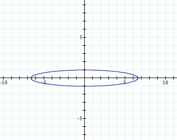
Open this graphing calculator file to view an animation of the graph. The animation reveals that as the n-value changes, the graph looks like an ellipse rather than a circle with radius 1. In particular, the shape is an ellipse that is "stretched" along the x-axis. This should make sense because the x-value corresponds to the cosine function, which is what is being changed in this example.
Example: x = cos(t) and y = n sin(t). Let n vary from -10 to 10. Here's a snapshot of the resulting change:
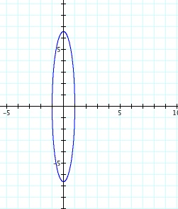
Open this graphing calculator file to view an animation of the graph. The animation reveals that as the n-value changes, the graph looks like an ellipse rather than a circle with radius 1. In particular, the shape is an ellipse that is "stretched" along the y-axis. This should make sense because the y-value corresponds to the sine function, which is what is being changed in this example.
What would happen if we let the equations be: x = cos(at) and y = sin(bt), where a is not equal to b?
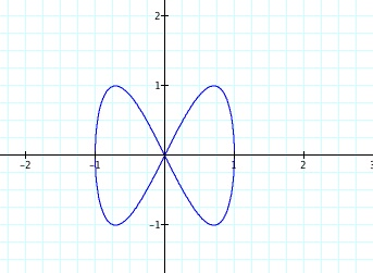
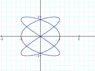
Example: Let x = cos(t) and y = sin(2t)
Example: Let x = cos(t) and y = sin(3t)
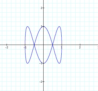
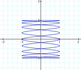
Example: Let x = cos(t) and y = sin(7t)
The changes that are being made are altering the shape of the graph. We see that instead of a unit circle, we have a graph with some number of loops. My conjecture is that changing the b-term affects the number of loops. If b is an interger value, then there will be b number of loops. Explore the Graphing Calculator file to see that this looks like the case.
Now what happens if we change the a-value? Do we expect the same results? Let's explore with examples.
Example: x = cos(2t) and y = sin(t)
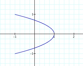
So, the graph looks like a parabola that opens to the left. Interesting. Let's try a few other examples.
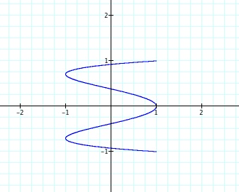
Example: x = cos(4t) and y = sin(t)
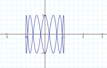
Example: x = cos(9t) and y = sin(t)
The changes that are being made are altering the shape of the graph. Explore the Graphing Calculator File to see that now the change and the number of loops is occuring along the y-axis.
Now what happens if we change both a and b? Let's explore a few more examples:
Example: x = cos(3t) and y = sin(2t)
Example: x = cos(3t) and y = sin(5t)
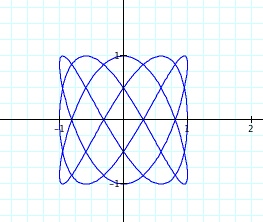
My knowledge regarding parametric curves is quite limited, so I enjoyed being able to use Graphing Calculator to make a few conjectures about the varying graphs and identify any pattern. It was interesting to see how changing the values in the equations affected the graphs. The graphs produced were unexpected -- instead of a unit circle, the graphs had varying number of loops and different shapes.