Assignment 10: Exploration of Trigonometric Parametric Equations

By: Mary Wisniewsky

In this assignment, we are going to take a look at different forms of the following parametric equations using the graphing calculator:

Introduction

In order to comprehend what the graph is going to look like for this set of parametric equations, lets go over the concept of a parametric equation.

A parametric curve consists of two functions on the plane x(t) and y(t). These functions describe the (x,y) coordinates in respect to a parameter t. These equations are widely used in areas of physics for range of motion or in trigonometry or many other areas of mathematics.

For example, if we let x(t)=t+1 and y(t)=2t, when t=1, then (x,y)=(2,2) on the cartesian plane. When you set it to an interval like 0 ≤ t ≤ 5, then the graph should appear as such:

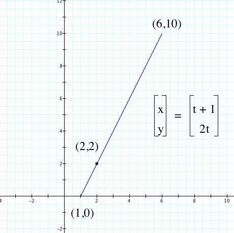
Here we have a linear line on the interval 0 ≤ t ≤ 5. We could rewrite these equations as one linear equation. In order to set up a linear equation, we need the slope and the y-intercept of the line. So to find the slope lets take two points, (1,0) and (2,2). If we find the change in y divided bythe change in x, then we should get for our change in y equal to 2 and our change in x equal to 1. Therefore the slope is 2.

So for our linear equation we have y=0.5x+b. To find b, we can plug in one of our points on the line to solve for b. Let's use (2,2):

y=2x + b

2=2(2) + b

2=4+b

b=-2

Thus, the linear equation represented for this parametric equation (with no interval on t) is

y = 2x-2

Now, Let's explore our original parametric equations:

x=cos t

y=sin t

What do you expect to see on the graph for these two functions?

Consider the interval 0 ≤ t ≤ 2π. For the following t values, we get

• For t=0, x=cos 0=1, y=sin 0=0; (1,0)
• For t=π/2, x=cos (π/2)=0, y=sin (π/2)=1; (0,1)
• For t=π, x= cos π=-1, y=sin π=0; (-1,0)
• For t=(3π/2), x=cos (3π/2)=0, y=sin (3π/2)=-1; (0,-1)
• For t=2π, x=cos (2π)=1, y=sin (2π)=0; (1,0)

These coordinates look very similar to coordinates for the unit circle. Now take a look at the graph:

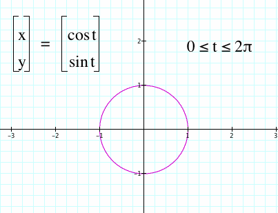
And the graph is identical to the standard unit circle. Therefore using this set of parametric equations can help generate various coordinates on the unit circle.

What will happen to the graph if the x and y functions are switched around?

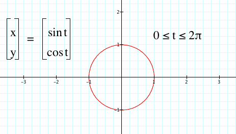
It still remains the same graph for this standard interval.

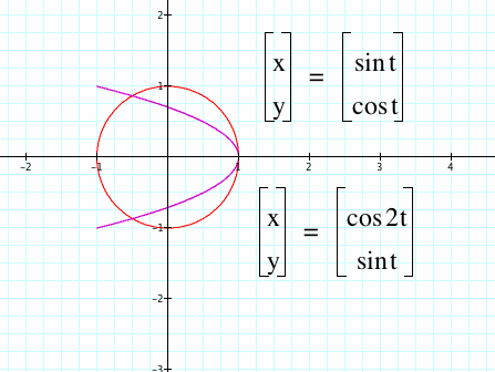
Now let's take a look at various forms on this equation. What if we changed the form of x(t) to x(t)=cos at.

Here we have in red the original graph and in pink is the altered graph of x(t) for 0 ≤ t ≤ 2π. Instead of having a full completion of a circle, the graph resembles a rotated parabola. Even if we changed our interval and increased the end boundary on the interval, the graph would not change shape.

0 ≤ t ≤ 2π

0 ≤ t ≤ 6π

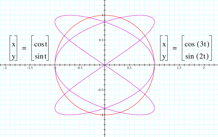
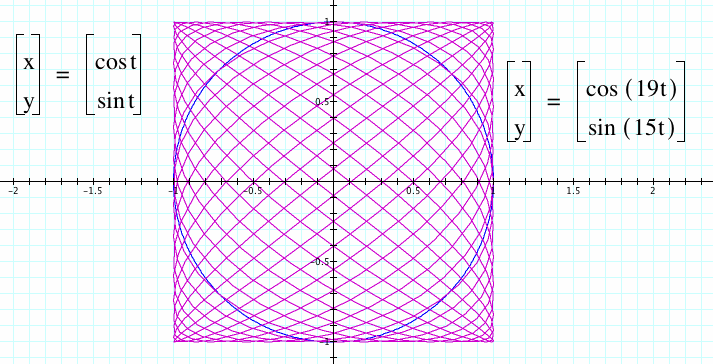
When we start to manipulate also the y(t) function in the parametric equations, we start to notice the main shapes and curves that can be formed from increasing a, b in

x(t)=cos at

y(t)=sin bt.

When the values of these a and b are changed, the numbers of curves and spirals increase.

Check out this video:

In red, you can see the original graph. In pink, you can see how x(t) is affected by the parameter n on a of x(t)=cos at. In blue, you can see how y(t) is affected by the parameter n on b of y(t)=sin bt. As n increases, the number of curves and spirals increases. For the pink equation, the curve is shifting and increasing in respect to the "x-axis" on a cartesian plane which makes sense since x(t) is the function with the parameter. For the blue equation, the curve is shifting and increasing in respect to the y-axis on a cartesian plane which makes sense since y(t) is the function with the parameter.

Now let's see the effect the original parametric equations with the form of:

x(t)= a cos t

y(t)= b sin t

Take a look at the following graph where in blue we have the original graph and in the pink a in x(t) is 2.

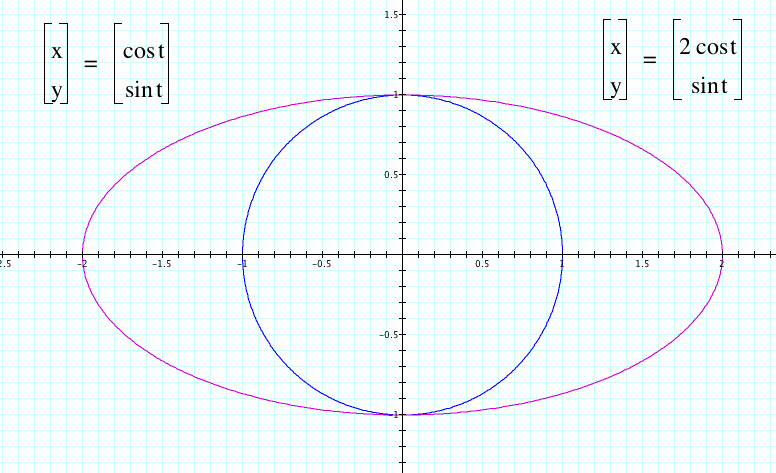
See how once a was increased, the graph stretched with respect to the x-axis. Should we expect the same if b is altered for y(t)?

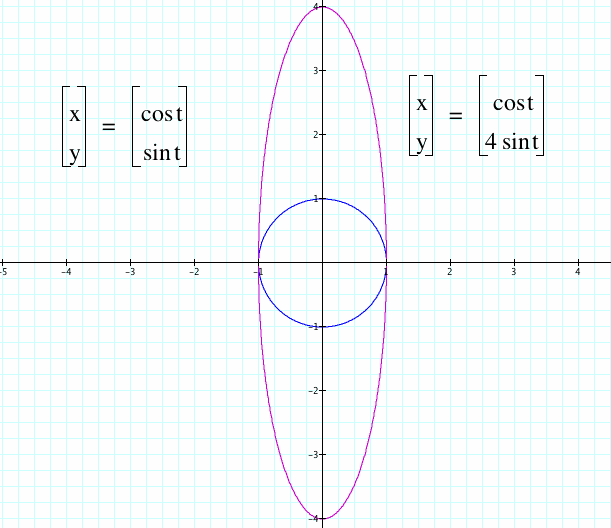
Instead of the curve being stretched with respect to the x-axis, the curve is stretched with respect to the y-axis. So, as a increases, the curve stretches horizontally on the x-axis, which correlates to the fact that x(t) is being altered. Also as b increases, the curves stretches vertically on the y-axis, which correlates to the fact that y(t) is being altered.

See the video to see how the graph changes as a and b are increasing and decreasing.

In conclusion, setting a parameter and manipulating the original parametric graphs can drastically changed the shape of the graph.

Explore further into these equations by looking at this movie of the animation of these equations or exploring on the graphing calculator app

Return to Mary Wisniewsky's main page