Exploring Quadratic and Cubic Functions.
By Raynold Gilles.
Exploring Quadratic and Cubic Functions.
By Raynold Gilles.
The Problem asks us to investigate Quadraric Equations for different values of a, b and c.
We will first consider the graph of y = x2 + bx + 1 for different values of b. These graphs were constructing using graphing Calculator lite.
In order to illustrate the effect caused by varying values of b, we varied values of b between -10 and +10.
![]()
![]()
![]()
![]()
![]()
![]()
![]()
![]()
![]()
After investigation one can notice that varying the values of b has the following effects:
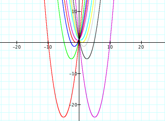
1. Translation
Positive values of b translate the vertex of the graph of our parabola to the left. Negative values of b on the other hand translate our graph to the right. It has to be kept in mind that the graphs are being translated vertically and horizontally simiulataneously.
As the absolute value of of b grows, the graph is translated down. Translating the graph affects our parabola's x interecept.
For values of b with an absolute value less than 1, our parabola does not intercept the y axis. This can be interpeted as a quadratic equation with imaginary solution where the discriminant isnegative.
For values to absolute value of two, there is a double solution equal to 1 when b is equal to -2 and equal to -1 when b is equal to 2. In both of these cases, our discriminant would be equal to zero.
As the Values of b become greater than 2 in absolute value, our parabola intercepts the y axis in two distinct points that are symmetric to the axis of symmetry. This can be interpreted as two real solutions with a positive disriminant.
The axis of symmetry in the case where a=1 can be computed by (-b/2).
We Will beging by changing the value of "b". to "y".
Below is the Graph of our parabola in the xb plane.
Therefore our equation is ![]()
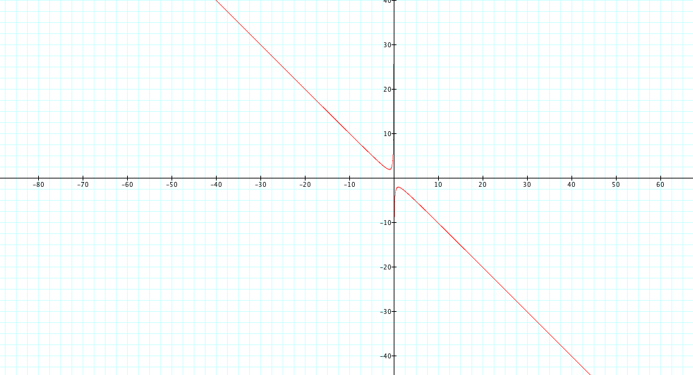
The graph above suggests that we created a Hyperbola that has the y axis as a horizontal asymptote and the line y=x as a slant asymptote.
Now that we have created our hyperbola, we will investigate the effects of varying values of c.
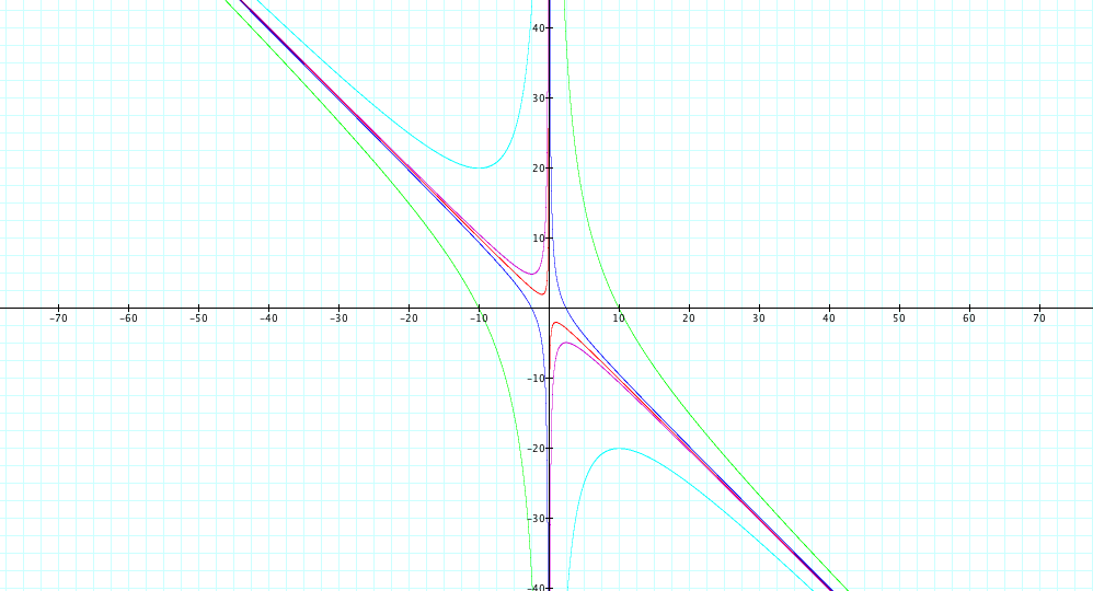
Looking at the image below for different values of c in the xb plane, we can make the conclusions that follow:
Negative values of c results in the hyperbola being asymptotic to the "y" axis in either the first or third quadrant.
Positive values of c result in the hyperbola being asymptotic to the "y" axis in either the second or fourth quadrant.
Similarly, Negative value of c results in our hyperbolas being asympotic to the line y=x in the quadrants in which they are not asymptotic to the y axis.
The next observation that one can make is that our hyperbolas tend to have vertices that are further away from the origin as the absolute value of c increases. The next obervation that can be made is that the curvature of our hyperbola is greatly affected by the values of c. This curvature is called "eccentricity" in geometry.
For example, the green graph where the value of c is 100 is straighter than the blue graph where the value of c is equal to 6.
Investigation 3: Investigating the equation of a third degree polynomial in the form:
The following important observation has to be made: The Maximum number of turning points is 2. This was observed after animating our graph using slider values on graphing calculator.
3.1.Investigating for different values of "a".
First we will focus on the cases where a are 1 and -1
The graph are symmetric around the origin. Furthermore, the two graphs are reflections of each other around the origin. One can therefore conclude that changing the sign of "a" reflects the a graph of the form
around the origin.
Let us further investigate our function by looking at the graph below.
We investigated the equation for different values of a as follow:
The following conclusion can be made:
The graph increases faster as the absolute value of a increases. This is normally called a vertical strech in mathematical language.
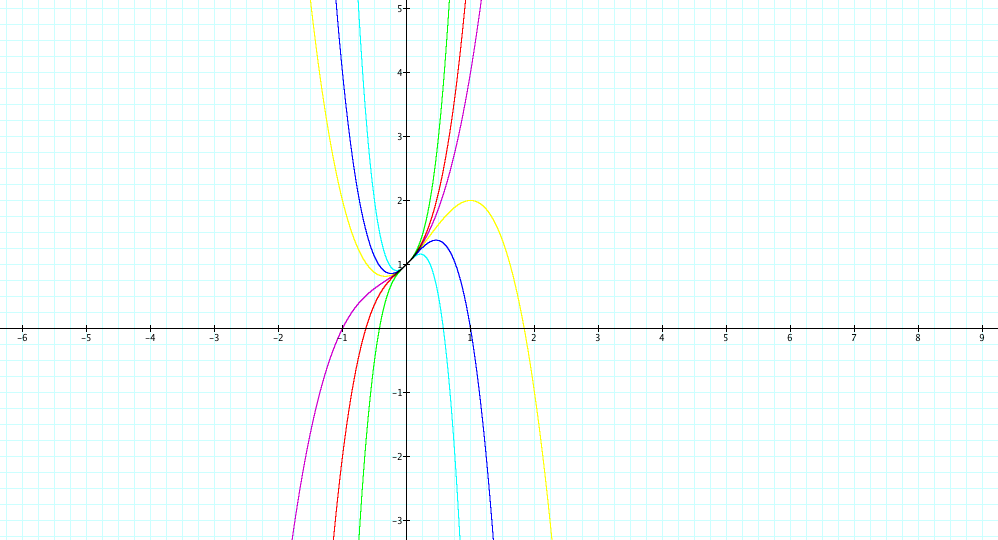
3.2.Investigating for different values of "b".
Below are the equations for different values of b that we investigated.
Investigating this graph leads us to the following conclusions:
Holding every other coefficient constant, positive values of "b" lead to a local maximum. The ordinate of our local maximum increases as the absolute value of "b" increases.
Holding every other coefficient constant, negative values of "b" lead to a local minimum. The ordinate of our local minimum decreases as the absolute value of "b" increases.
Simply said, our absolute minimum or maximum gets further and further away from the x asis as the absolute value of b increases.
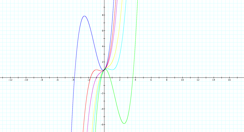
3.3.Investigating for different values of "c".
Our next step was to hold the values of a and be constand while varying the values of c.
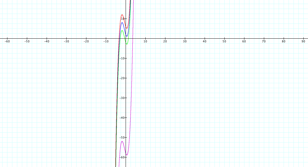
Keeping in mind that a positive value of b lead to a local maximum, we set our value of b equal to "2".
Below is a graph with different values of c
.
Negative values of c lead to both a local maximum and mimimum while positive values of c lead to neither a local maximum nor a local minimum. When it comes to negative values, the larger the absolute value of c, the further away is the absica of our maximum or minimum.
3.4.Investigating for different values of "d".
Changing the values of d result in a translation of our graph. This can be observed below for four different values of "d".
The purple graph above is the one where "d" is equal to 1. As the value of d changes to 2, the graph shifts vertically up.
Similarly, as the value of d changes to 6, our graph shifts vertically . One can also observe that the value of d determines the value of our y intercept. For example the y intercept is (0,2) when d is equal to 2 and (0,6) when d is equal to 6.