| This is the 3rd part of my write-up of Assignment #11 |
Brian R. Lawler
|
| EMAT 6680 |
12/14/00
|
The Problem
| Investigate varying a, b, c, and k. |
|
|
|
|
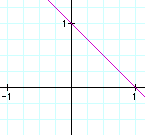
Here is a picture of the graph of As I varied the value of c, the graph moves away from the origin, with the line seemingly equivalent toy = -x + c. Click on the graph itself to investigate this behavior on your own. |
 |
|
|
a had a sort of tilting effect. If you notice from above, this relation has an x-intercepts of (c/a, 0). As a changes, this intercepts remains, but the graph rocks - or rotates around this intercept. (Note: in each of the previous cases, I have only changed one variable. Very interesting complexities are introduced with k, but I will ignore these until later. For now, the discussions I have presented are general enough to be always true.) b also has a sort of tilting effect, but in a different orientation. As b changes, the graph rocks around the point (0, c/a). If a and b are varied together, the behavior is much like c above. The graph will appear as a straight line, traveling in and away from the origin. |
||
|
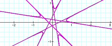
Then, as k changes, it adds a dimensions, or bends to the line, introducing new lines from the left and right. Click here to further investigate a graph set up to observe this particular behavior. |
||
| And finally, k has a rather interesting effect. When k = 0, the relation is a radius c circle centered at the origin. | |
| k = 0.1 | 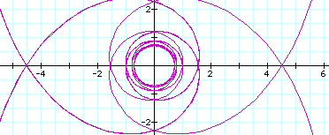 |
| k = 0.2 | 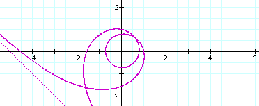 |
| k = 0.333 | 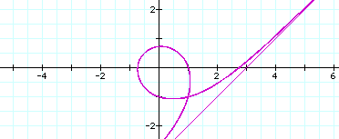 |
| k = 0.4 | 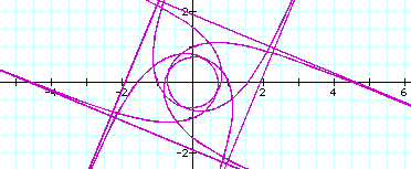 |
| k = 0.5 | 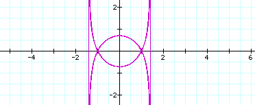 |
| k = 0.6 | 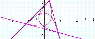 |
| k = 0.9 | 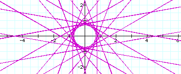 |
| k = 2 | 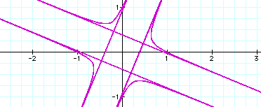 |
| k = 3 | 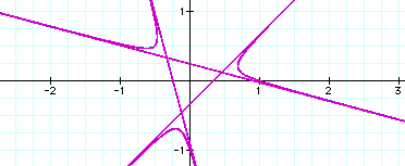 |
|
k = 5 |
 |
|
As can be seen above, k has a sort of rotating and multiplying property. The other coefficient's primarily affect the scale of the shape. As a final note, all the graphs above were completed with a domain of theta to be from 0 to 100. I did this to see a larger picture of what may be happening. The final step I took with looking at this graph was to attempt to observe how these graphs get traced out. To do this, I adjusted the domain. Below is a movie of k varying from -5 to 5, with only a domain of 0 to 2pi. With a limited domain, it becomes more apparent how the relation is drawn. |
|
Reflections
There are clearly observations I was able to make regarding these polar equations that could not be so readily observed without a tool such as Graphing Calculator 3.0. The dynamic relation grapher allows for immediate feedback on changing parameters. This can spark interest to understand further why the parameter has the observed effect. I suspect this develops a greater symbolic reasoning skill for the learner as well as a stronger connection between a graphical and symbolic representation of these relations. Additionally, learners can act more as inquirers, conjectures, discoverers, reasoners, arguers, etc... I don't think there would ever be a learning expectation for a student to spit back the effect of b in the particular equation above. Instead, the learner is equipped to be flexible understanding more about any type of polar (and other) equation they may come across. I look forward to someday observe a teacher (or a curriculum) use this tool in the type of manner described above.
 |
Comments? Questions? e-mail me at blawler@coe.uga.edu |
| Last revised: December 28, 2000 |
|