Write-up #12

Using Excel to Explore Stamps Data

by

Holly Anthony

Problem:

The data in this exploration is based on the first class letter postage for the US Mail from 1919 to 1994. I will plot the data and develop a prediction function and use this function to predict:

• what year first class postage will cost $1
• when it will cost 64 cents, and
• how soon we should expect the next 3 cent increase.

Entering our Data in Excel

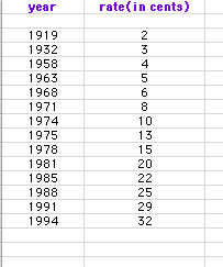
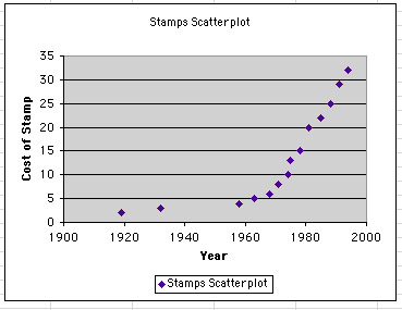
Let's begin by entering our data into an Excel spreadsheet and graphing the data set in a scatterplot.

Stamp Data Spreadsheet

Stamp Data Scatterplot

Finding a Function to Model our Data

Now, let's find a function that best fits the given set of stamp data. From looking at the curve of the data in the above scatterplot, it appears to be either an exponential function or a power function. ( Finding the curve of best fit is not going to be easy since the curve is slow to take off.)

Using a graphing calculator, I found the exponential regression function to be:

y = .0066456427(1.039760577^x)

Using a graphing calculator, I found the power regression function to be:

y= .00007268463(x^1.733522632)

Let's use these equations with our given x-values (years) and graph them with our data set to see which of these functions best represents our actual data set most closely.

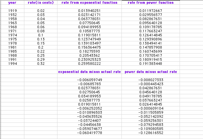
Below is our new Excel spreadsheet with the data entered from these two equations.

It is important to note that we have left out the '19' in each date when calculating our data.

Stamp Data with Function Data

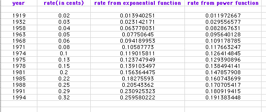
From looking at the data in the spreadsheet, it is difficult to determine which function most closely represents our actual data. Let's look at the graphs of the two functions with our data.

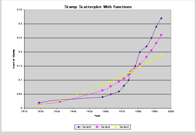
Notice that our actual data is represented by the dark purple line. The exponential function data is represented by the pink line and the power function data is represented by the yellow line. From looking at the graphs, it is still difficult to determine which function best fits our data, so let's examine the residuals.

First, I found the difference (called the residuals) between the function-produced data and the actual data. Since some of the residuals are positive and some of the residuals are negative, it was not a good idea to average the residuals at this point, so I squared the residuals in order to get a set of positive numbers and then I averaged the squares.

The following spreadsheets show the residuals for the exponential function and for the power function.

Measure of Error using Residuals

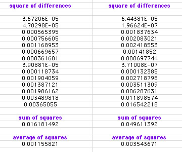
Notice that the average of the squares for the exponential function is approximately 0.00116 and the average of squares for the power function is approximately 0.00354. The closer these values are to zero, the "better" the function is at modeling the data. I will therefore choose the exponential function as the 'best' function to model this data. (Note: this model may not be the best possible, but it is the best I could find. A better function for modeling this data could be found by omitting the 1919 data point (outlier).

Our function: y = 0.0066456427(1.039760577^x)

Using Our Function to make Predictions

Now that I have decided on the exponential function as the 'best' function to model this data, I can use it to predict:

• what year first class postage will cost $1
• when it will cost 64 cents, and
• how soon we should expect the next 3 cent increase.

Using the function: y = 0.0066456427(1.039760577^x), I found the following:

• In the year 2029, postage will cost $1
• In the year 2017, postage will cost 64 cents, and
• In the year 1996, we can expect the next 3 cent increase (based on the data given; obviously we are past 1996!)

(Obviously, these are approximations since our function is not 'truly' the 'best' function to model this data.) A better prediction function could be found by eliminating the 1919 data point (an outlier).

Return to Main Page