It has now become a rather standard exercise, with availble technology, to construct graphs to consider the equation

and to overlay several graphs of

for different values of a, b, or c as the other two are held constant. From these graphs discussion of the patterns for the roots of

can be followed.

If we set   
                      
for  a= -3, -2, -1, 0, 1, 2, 3, and overlay the graphs , the following picture is obtained.

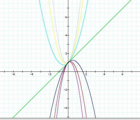
We can discuss the "movement" of a parabola as  a  is changed. The parabola always passes through the same point on the y-axis ( the point (0,1) with this equation). For a < 0 the parabola will go down with two real roots. For a = 0, the equation become the linear equation. For  a> 0, the parabola will go up.

if we set

for b = -3, -2, -1, 0, 1, 2, 3, and overlay the graphs, the following picture is obtained.

We can discuss the "movement" of a parabola as b is changed. The parabola always passes through the same point on the y-axis ( the point (0,1) with this equation). For b < -2 the parabola will intersect the x-axis in two points with positive x values (i.e. the original equation will have two real roots, both positive). For b = -2, the parabola is tangent to the x-axis and so the original equation has one real and positive root at the point of tangency. For -2 < b < 2, the parabola does not intersect the x-axis -- the original equation has no real roots. Similarly for b = 2 the parabola is tangent to the x-axis (one real negative root) and for b > 2, the parabola intersets the x-axis twice to show two negative real roots for each b.

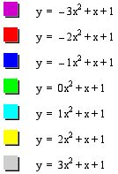
if we set
                   

for c = -3, -2, -1, 0, 1, 2, 3, and overlay the graphs, the following picture is obtained.

We can discuss the "movement" of a parabola as c is changed. The parabola always has the same shape and the graph go up as c increases and go down as c decreases.

After looking at the graph of   in the xa plane, the xb plane, and xc plane after holding the other two  constant, you can generalize the properties of the roots of the original equation in the graph.

If we take any particular value of a, say a = 1,-1 and 0.25, and overlay this equation on the graph we add a line parallel to the x-axis. If it intersects the curve in the xa plane the intersection points correspond to the roots of the original equation for that value of a. We have the following graph.
 

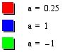
For each value of a we select, we get a horizontal line. It is clear on a single graph that we get one negative  and one positive real roots of the original equation when a < 0, one negative real root -1 when a = 0, two negative real roots for 0 < a < 0.25, One negative real root when a=0.25 , and  no real roots when a >  0.25.
 

Graphs in the xb plane.

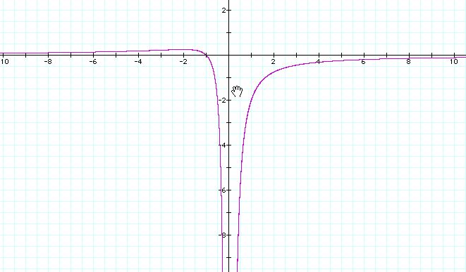
Consider again the equation

Now graph this relation in the xb plane. We get the following graph.

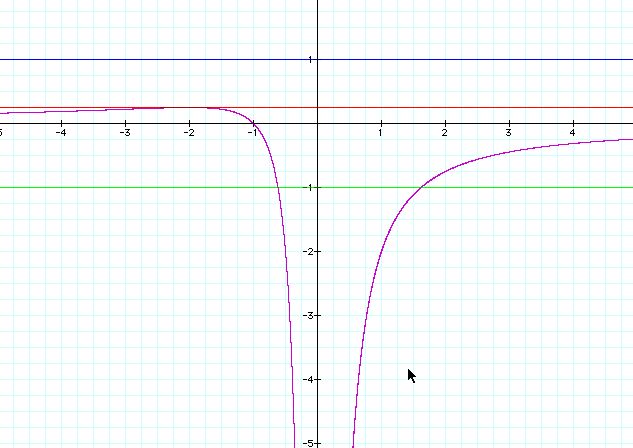
If we take any particular value of b, say b = 3, and overlay this equation on the graph we add a line parallel to the x-axis. If it intersects the curve in the xb plane the intersection points correspond to the roots of the original equation for that value of b. We have the following graph.

For each value of b we select, we get a horizontal line. It is clear on a single graph that we get two negative real roots of the original equation when b > 2, one negative real root when b = 2, no real roots for -2 < b < 2, One positive real root when b = -2, and two positive real roots when b < -2.

Consider the case when c = - 1 rather than + 1.

For each value of b, we always get one positive and one negative real roots of the original equation.

Graphs in the xc plane.

is considered. If the equation is graphed in the xc plane, it is easy to see that the curve will be a parabola. For each value of c considered, its graph will be a line crossing the parabola in 0, 1, or 2 points -- the intersections being at the roots of the orignal equation at that value of c. In the graph, the graph of c = 1 is shown. The equation

will have two negative roots -- approximately -0.2 and -4.8.

There is one value of c where the equation will have only 1 real root -- at c = 6.25. For c > 6.25 the equation will have no real roots and for c < 6.25 the equation will have two roots, both negative for 0 < c < 6.25, one negative and one 0 when c = 0 and one negative and one positive when c < 0.

Return to the Top