
In countless algebra 1 classrooms all across America, teachers show their students the standard form of a quadratic equation and then explain various ways of finding its roots. However, one thing that doesn't always happen in these classrooms is an explanation of the relationship between the standard form of the quadratic equation and its roots. That is, how do the coefficients a,b, and c effect the roots of a given equation? Can you tell just by looking at an equation whether it will have real roots, or imaginary roots? Can you tell how many roots there will be, and if so, will they be positive, or negative?
If you answered yes to any of the preceding questions, then you probably teach your students about the discriminant and how it can be used to determine the number and type of roots of a given quadratic. Good for you. What follows here is a way to show the relationship of the discriminant graphically using some simple algebra and a graphing calculator program such as Graphing Calculator. If you answered no to the above, allow me to drop some knowledge on you.
First of all, lets review exactly what the
discriminant is. In the quadratic formula, the discriminant is
the part under the radical sign. Namely, ![]() .
The standard algebra 1 text will state that when the discriminant
is positive, then there will be two real roots of the equation.
If the discriminant is zero, there will be one real root, and
if the discriminant is negative, this indicates no real roots.
This is all well and good, but I believe our teaching would be
more powerful if we could show this relationship visually in a
way that makes the concept behind the "rule" make sense.
.
The standard algebra 1 text will state that when the discriminant
is positive, then there will be two real roots of the equation.
If the discriminant is zero, there will be one real root, and
if the discriminant is negative, this indicates no real roots.
This is all well and good, but I believe our teaching would be
more powerful if we could show this relationship visually in a
way that makes the concept behind the "rule" make sense.
To accomplish our goal, we are going to
have to look at the graphs of quadratic equations in a different
way. Instead of graphing in our normal xy plane, we are going
to look for relationships between a, b, and c in the xb plane.
That is, the horizontal axis will represent the x variable, and
the y axis will represent the variable b in ![]() .
This means we will really be working with equations
of the form
.
This means we will really be working with equations
of the form ![]() . What we would like to do is examine
each of the cases described in the text from an algebraic standpoint,
and then show these same relationships graphically. So, let's
begin...
. What we would like to do is examine
each of the cases described in the text from an algebraic standpoint,
and then show these same relationships graphically. So, let's
begin...
If ![]() > 0, then we know
> 0, then we know
![]() >
> ![]() . Taking the square
root of both sides we find that b > +/-2
. Taking the square
root of both sides we find that b > +/-2![]() .
But. because this is a compound inequality, we need to split it
into two inequalities. These will be b > 2
.
But. because this is a compound inequality, we need to split it
into two inequalities. These will be b > 2![]() ,
or b < -2
,
or b < -2![]() . So, in order for an equation
to have real roots, a, b, and c will have to satisfy these equations.
Let's look at some graphs of quadratic equations in the xb plane
that fit these inequalities and see what is really happening.
. So, in order for an equation
to have real roots, a, b, and c will have to satisfy these equations.
Let's look at some graphs of quadratic equations in the xb plane
that fit these inequalities and see what is really happening.
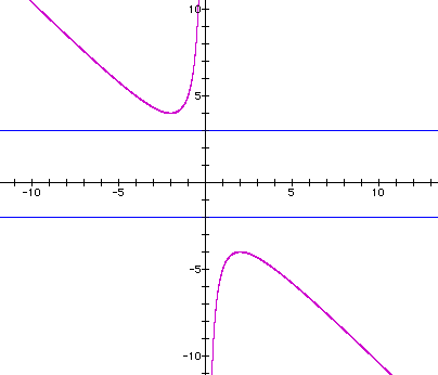
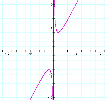
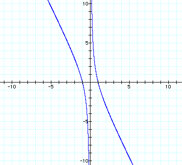
Case 1 - Both a and c are positive
Below is a graph of the equation ![]() (remember
we are in the xb plane so we can look at how a and c relate to
b.)
(remember
we are in the xb plane so we can look at how a and c relate to
b.)
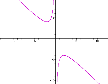
There will be real solutions to this equation whenever any horizontal line, representing the value of the b variable, intersects the graph. For example, the line b= 5 will intersect the graph in 2 points. These points of intersection are the two roots of the equation for b =5.
We can see that for any value of b > 4, we will get two real solutions for x and they will both be negative. In the above example, when b = 5, the two roots are x = -4 and x = -1.
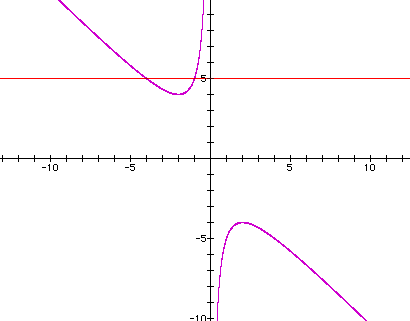
You may also notice that we will also get two solutions when our horizontal line intersects the bottom half of the hyperbola. That is, when x < -4. For example, using the line b = -6, we see below that it also intersects in two places indicating two real roots. In this case, both roots are positive. (approximately, x = .76392 and x = 5.23607)
Now, let's go back to our original equation
in standard form and check our "rule". Remember that
the rule says we should get two real roots when For ![]() ,
a = 1 and c = 4. Substituting into our compound inequalities implies
that b > 2
,
a = 1 and c = 4. Substituting into our compound inequalities implies
that b > 2 ![]() or b < -2
or b < -2 ![]() ,
which means b >4 or b < -4. Remarkably, or maybe not so,
these were the same parameters we decided on based upon our graphs.
But, in addition to this information, the graphs were also able
to tell us that when b >4, both of the solutions would be negative
, and when b < -4, both solutions will be positive. Nice!
,
which means b >4 or b < -4. Remarkably, or maybe not so,
these were the same parameters we decided on based upon our graphs.
But, in addition to this information, the graphs were also able
to tell us that when b >4, both of the solutions would be negative
, and when b < -4, both solutions will be positive. Nice!
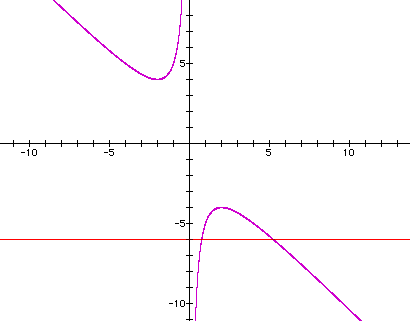
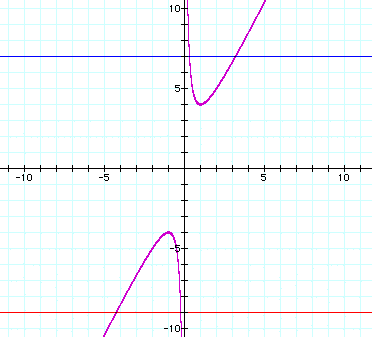
The second "rule" states that
when the discriminant is zero, then there will be one real root.
Algebraically, this means that .![]() We can
explore the second "rule" using the same graphs as above.
From the graph below we can find a horizontal line that is tangent
to the upper half of the hyperbola at its vertex, as well as one
that is tangent to the bottom half at its vertex.
We can
explore the second "rule" using the same graphs as above.
From the graph below we can find a horizontal line that is tangent
to the upper half of the hyperbola at its vertex, as well as one
that is tangent to the bottom half at its vertex.
These two lines are the lines b = 4 and
b = -4. They are tangent to![]() , each
at the vertex of the curve. When b = 4, we get one real root that
is negative, namely x = -2. When b = -4, then we get one positive
root, that is, x = 2. To verify our finding algebraically,using
the "rule", we substitute our values for a and c into
, each
at the vertex of the curve. When b = 4, we get one real root that
is negative, namely x = -2. When b = -4, then we get one positive
root, that is, x = 2. To verify our finding algebraically,using
the "rule", we substitute our values for a and c into
![]() .In doing this, and solving for b, we see
that either b =4 or b = -4. Once again, the graph is not only
giving us a visual of this, but also helping determine the sign
of the solution.
.In doing this, and solving for b, we see
that either b =4 or b = -4. Once again, the graph is not only
giving us a visual of this, but also helping determine the sign
of the solution.
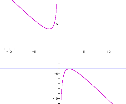
The third "rule" refers to no
real solutions when ![]() < 0. Algebraically,
we can show, using the same argument as above, that this implies
that there will be no real solutions when b < 2
< 0. Algebraically,
we can show, using the same argument as above, that this implies
that there will be no real solutions when b < 2![]() and when b > -2
and when b > -2![]() . Looking at the graph
of
. Looking at the graph
of ![]() , we can see that the horizontal
lines for b, where - 4 < b < 4, will never intersect either
of the hyperbolas. For example, the lines b = 3 and b = -2, shown
below, imply that there are no real solutions to our equation
for either of those values of b.
, we can see that the horizontal
lines for b, where - 4 < b < 4, will never intersect either
of the hyperbolas. For example, the lines b = 3 and b = -2, shown
below, imply that there are no real solutions to our equation
for either of those values of b.
Verifying the rule algebraically we can
substitute and find that there are no real roots for the equation![]() when b <2
when b <2![]() , and when
b >-2
, and when
b >-2![]() . Simplifying these expressions,
we see the rule indicates no real solutions for -4 < b <4.
. Simplifying these expressions,
we see the rule indicates no real solutions for -4 < b <4.
Case 2 - Both a and c are negative
Now we will look at an example where both
a and c are negative. Let's look at the equation ![]() ,
and its graph.
,
and its graph.
Once again, in the xb plane, we will have a solution any time a horizontal line intersects either half of the hyperbola. So for any values of b > 4 or b < -4, we should get two solutions. So if , for example, b = 7, or if b = -9, we would get two points of intersection that would symbolize the roots for that given equation.
In the case of b = 7, we see that there are two positive values for x, approximately x = .313, or x = 3.19. However, when b = -9, we get two negative values for solutions. This is exactly the opposite of what we found when both a and c were positive. This makes sense of course, since that if a and c have the same sign, then -4ac will always have the same sign. This implies the solutions will either both be positive or both negative. Changing the signs of a and c simply reflected the graph across the axis, which in turn changed when the solutions will be positive or negative.
From the "rule", we should see
that we get two real roots when b > 2![]() and when b < -2
and when b < -2![]() . In this particular
case, substitution shows us that b >4 or b < -4, exactly
what the graph shows.
. In this particular
case, substitution shows us that b >4 or b < -4, exactly
what the graph shows.
We could repeat the above arguments to show the graph and the "rule" agree for one solution, or no solutions as well. In this case, one solution when b = 4 or b = -4, no solutions for -4 < b < 4.
Case 3 - a and c have different signs
This case is a bit different
that the first two. Let's look at two different equations, ![]() and
and ![]() .
.
You should notice that the graphs in the xb plane are still hyperbola, but these are much more shallow than the other graphs we have seen. This shallowness will have a big effect on our solutions. If we draw any horizontal line in either of these graphs, we will see that it will always have two intersections, and therefore two solutions. In both cases, there will be one solution that is positive and one solution that is negative. If we think about this algebraically using our "rule" we can see that this conclusion makes sense.
If a and c have different signs, then the
value of -4ac will always be positive. So we will get two solutions
if  > 0. If this is true, then we know
 ![]() >
-
>
-![]() . Since b squared is always positive, we know
that this inequality will be true for any value of b.
. Since b squared is always positive, we know
that this inequality will be true for any value of b.
So, we have shown the graphical representations of the discriminant as a function of number of solutions. This will help students to build a better understanding of the mathematics behind solving quadratics. This will make them leaders of the classroom, not just followers of a rule.