The following data is based on the first class letter postage for the US Mail from 1933 to 1966.
| YEAR | RATE (IN CENTS) |
| 1919 | 2 |
| 1932 | 3 |
| 1958 | 4 |
| 1963 | 5 |
| 1968 | 6 |
| 1971 | 8 |
| 1974 | 10 |
| 1975 | 13 |
| 1978 | 15 |
| 1981 | 20 |
| 1985 | 22 |
| 1988 | 25 |
| 1991 | 29 |
| 1994 | 32 |
| 1997 | 33 |
| 1999 | 34 |
| 2002 | 37 |
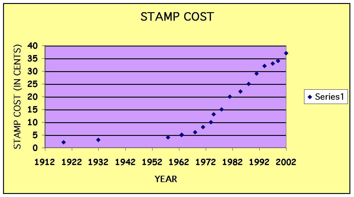
Lets look at the scatter plot of this data:

Does this function represent a linear model, log model, power model or an exponential model? Even though when we look at the scatter plot it appears to be exponential, but we can't just use our eyes to determine which model the data fits best.
Since a power function and an exponential function are pretty similar lets examine both models.
A power regression is in the form y=ax^b, by transforming the equation into a linear form we can look at the correlation coefficient. By looking at the correclation coefficient we are able to decide which model best fits the data, power or exponential.
Lets begin with our form for power function
y=ax^b
Take the log of both sides
log y = log (ax^b)
Use log properties to perform the following:
log y = log a + (b log x)
Let log y = Y and Let log a = A and log x = X
therefore, Y = A + bX, so now we have a linear form of the power function and we can use (log x, log y) to graph our data. By using (log x, log y) we can look at the correlation coefficient and determine if it is a good fit for the graph.
| log x | log y |
| 3.28307497473547 | 0.301029995663981 |
| 3.28600712207947 | 0.477121254719662 |
| 3.29181268746712 | 0.602059991327962 |
| 3.29292029960001 | 0.698970004336019 |
| 3.29402509409532 | 0.778151250383644 |
| 3.29468662427944 | 0.903089986991943 |
| 3.29534714833362 | 1 |
| 3.29556709996248 | 1.11394335230684 |
| 3.29622628726116 | 1.17609125905568 |
| 3.29688447553855 | 1.30102999566398 |
| 3.29776051109913 | 1.34242268082221 |
| 3.29841638006129 | 1.39794000867204 |
| 3.29907126002741 | 1.46239799789896 |
| 3.29972515397564 | 1.50514997831991 |
| 3.3003780648707 | 1.51851393987789 |
| 3.30081279411812 | 1.53147891704226 |
| 3.3014640731433 | 1.56820172406699 |
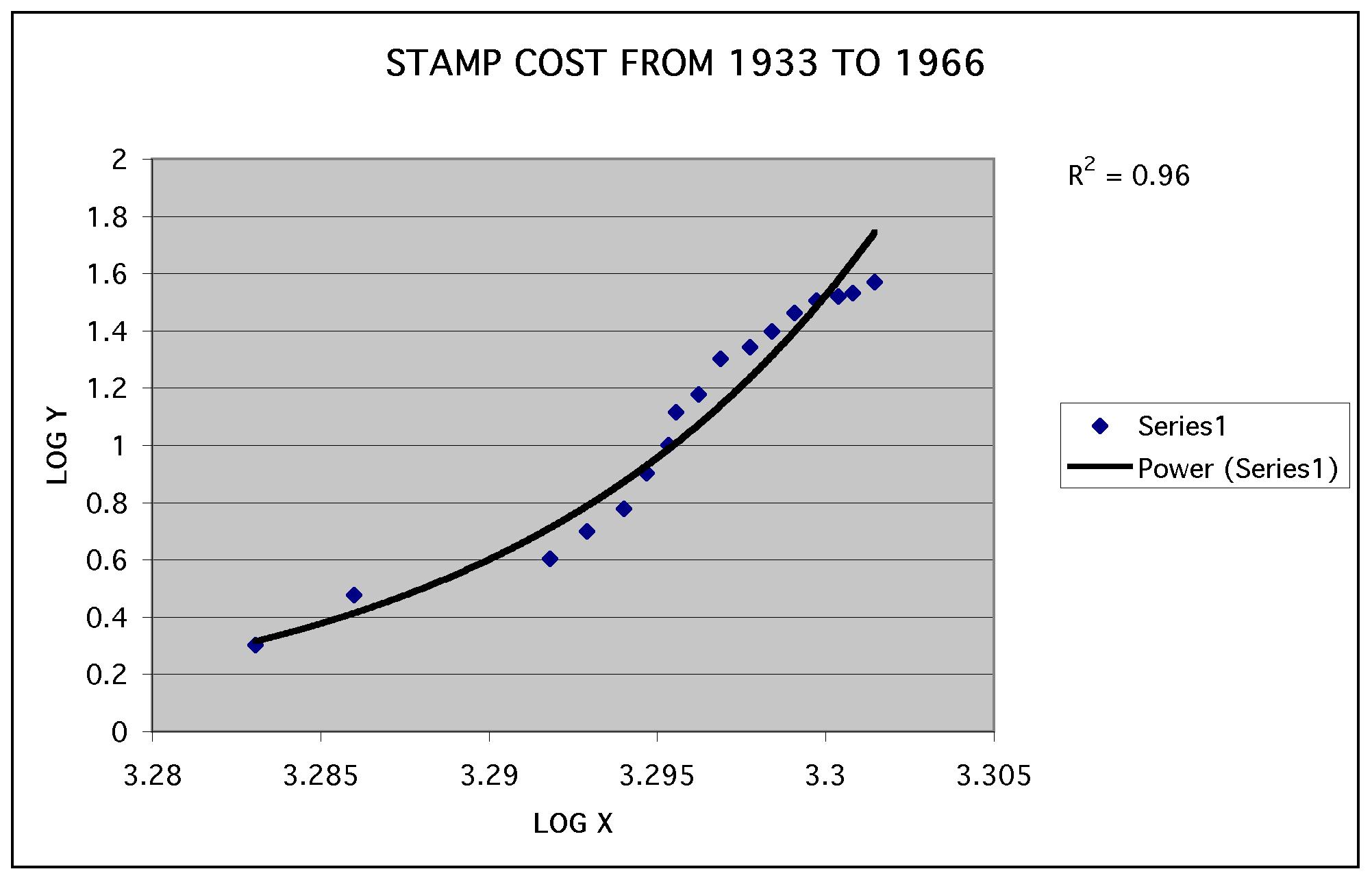
The graph below shows the power function of the stamp data using (log x, log y). We have drawn the trend line for the data and found the correlation coefficient which is 0.96. The closer the correlation coeffiicient is to one the better fit the data is.

Now lets look at the exponential model and see if its correlation coefficient better fits the model.
Exponential Function
Lets begin with the form y = ab^x
Take the log of both sides:
log y = log (ab ^x)
Use the properties of log to obtain the following:
log y = log a + x log b
Let log y= Y and log a = A and log b= B
then Y = A + Bx
therefore, Y = A + BX, so now we have a linear form of the exponential function and we can use ( x, log y) to graph our data. By using ( x, log y) and we can look at the correlation coefficient to determine if it is a good fit for the graph.
| year | log y |
| 1919 | 0.301029995663981 |
| 1932 | 0.477121254719662 |
| 1958 | 0.602059991327962 |
| 1963 | 0.698970004336019 |
| 1968 | 0.778151250383644 |
| 1971 | 0.903089986991943 |
| 1974 | 1 |
| 1975 | 1.11394335230684 |
| 1978 | 1.17609125905568 |
| 1981 | 1.30102999566398 |
| 1985 | 1.34242268082221 |
| 1988 | 1.39794000867204 |
| 1991 | 1.46239799789896 |
| 1994 | 1.50514997831991 |
| 1997 | 1.51851393987789 |
| 1999 | 1.53147891704226 |
| 2002 | 1.56820172406699 |
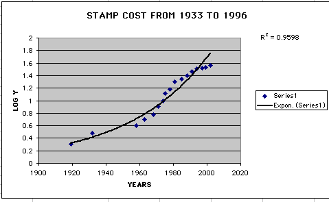
The graph below shows the exponential function of the stamp data using (x, log y). We have drawn the trend line for the data and found the correlation coefficient which is 0.9598. The closer the correlation coeffiicient is to one the better fit the data is.

Since the correlation coefficient of the exponential model and the power model are very close either model will work.
Now we need to find the equation that best fits the power function and the exponential function so we can use the equations to predict years and rates.
In order to find the equation we need to find the slope and y-intercept for our data.
To find the slope: Correlation Coefficient * (Standard Deviation of X divided by the Standard Deviation of y).
To find the y-intercept: Mean of y-Slope*Mean of x
The following spreadsheet shows how the standard deviation of x,y, slope and the y-intercept were calculated.
| year | rate(in cents) | X1-Mean | SQRED | Y1-Mean | SQRED |
| 1919 | 2 | -56 | 3136 | -15.52 | 240.8704 |
| 1932 | 3 | -43 | 1849 | -14.52 | 210.8304 |
| 1958 | 4 | -17 | 289 | -13.52 | 182.7904 |
| 1963 | 5 | -12 | 144 | -12.52 | 156.7504 |
| 1968 | 6 | -7 | 49 | -11.52 | 132.7104 |
| 1971 | 8 | -4 | 16 | -9.52 | 90.6304 |
| 1974 | 10 | -1 | 1 | -7.52 | 56.5504 |
| 1975 | 13 | 0 | 0 | -4.52 | 20.4304 |
| 1978 | 15 | 3 | 9 | -2.52 | 6.3504 |
| 1981 | 20 | 6 | 36 | 2.48 | 6.1504 |
| 1985 | 22 | 10 | 100 | 4.48 | 20.0704 |
| 1988 | 25 | 13 | 169 | 7.48 | 55.9504 |
| 1991 | 29 | 16 | 256 | 11.48 | 131.7904 |
| 1994 | 32 | 19 | 361 | 14.48 | 209.6704 |
| 1997 | 33 | 22 | 484 | 15.48 | 239.6304 |
| 1999 | 34 | 24 | 576 | 16.48 | 271.5904 |
| 2002 | 37 | 27 | 729 | 19.48 | 379.4704 |
| Total Sum Squared | 8204 | 2412.2368 | |||
| Divide by Sample | 512.75 | 150.7648 | |||
| Sx | 22.6439837484485 | Sy | 12.2786318456089 | ||
| Sx/Sy | 1.84417808377784 | ||||
| SLOPE | |||||
| POWER | 1.77041096042673 | ||||
| EXPON. | 1.77004212480997 | ||||
| Y-INTERCEPT | |||||
| POWER | 1943.98239997332 | ||||
| EXPON. | 1943.98886197333 |
Now let's take a look at the equation of the power function and the exponential function:
Power Function
Y = 1943.9823 + 1.77041096 X
Exponential Function:
Y = 1943.98886 + 1.77004212 X
Now we can use these equations to predict which year the stamp will reach $1.00.
Since the functions are so close it doesn't matter which one you choose.
When the cost of the stamp will be 64 cents?
How soon should we expect the next 3 cent increase?
Return to: Jennifer Weaver's Home Page