
It has now become a rather standard exercise, with available
technology, to construct graphs to consider the equation
and to overlay several graphs of
for different values of a, b, or c. From these graphs, discussion
of the patterns for the roots of
can be followed.
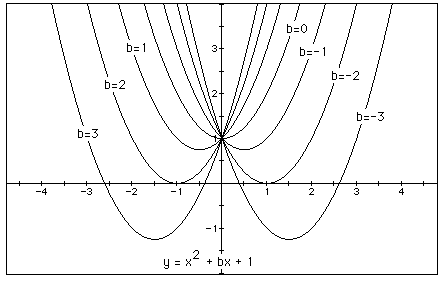
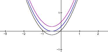
Let's first start by looking at different values of a. We will set b=1 and c=1 for
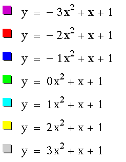
Now, we will explore a = -3, -2, -1, 0, 1, 2, 3
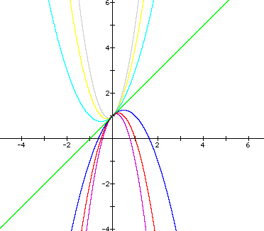
From the graph above, we can see that the equation when a=0 is tangent to all of the parabolas with a as a different values. We can also see that the line of tangency will always cross the y-axis at c with a slope of b since the equation of the line will be
When b=1 and c=1, our original equation will have two roots if a is negative. If a=0 our original equation will have one root. For each negative a value there are 2 roots, one positive root and one negative root. Notice if we changed the value of c then the a values that have roots would change. Now, it appears that our original equation will not have roots for positive a, but take a look at the next couple of equations.
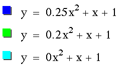
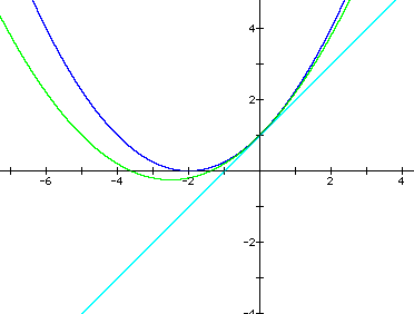
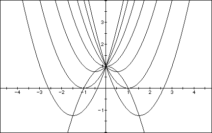
Here, we see that the our equation becomes tangent to the x-axis at (-2, 0) giving us one negative root for a=0.25 and two negative roots for 0<a<0.25.
Graphs in the xa plane.
Consider the equation
Now graph this relation in the xa plane. We get the following graph.
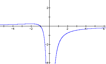
If we take any particular value of a, say a = -2, and overlay this equation on the graph we add a line parallel to the x-axis. If it intersects the curve in the xa plane, the intersection points correspond to the roots of the original equation for that value of a. We have the following graph.
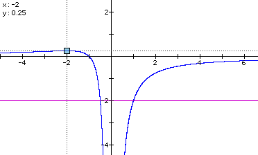
For each value of a we select, we get a horizontal line. It
is clear on a single graph that we get a negative real root and
a positive real root of the original equation when a<0, one
negative real root when 0 < a < 0.25, one negative real
root when a=0.25, and no real roots for a>0.25. This is exactly
what we discovered in our previous exploration of ![]() .
.
Next, let's explore b. We will set a=1 and c=1.
So, if we set
![]()
for b = -3, -2, -1, 0, 1, 2, 3, and overlay the graphs, the
following picture is obtained.
We can discuss the "movement" of a parabola as b is changed. The parabola always passes through the same point on the y-axis ( the point (0,1) with this equation). We know this holds for all values of a and b since substituting 0 for x gives us y = 1.
For b < -2 the parabola will intersect the x-axis in two
points with positive x values thus giving two positive real roots
for the original equation. For b = -2 , the parabola is tangent
to the x-axis so the original equation has one positive real root
at the point of tangency. For -2 < b < 2, the parabola does
not intersect the x-axis so the original equation has no real
roots. For b = 2 , the parabola is tangent to the x-axis providing
one real negative root. Finally, for b > 2, the parabola intersects
the x-axis twice to show two negative real roots.
Now, consider the locus of the vertices of the set of parabolas
graphed from
The vertices are as follows:
As you can see the locus of the vertices appears to be parabolic. To find the equation of the parabola we first go back to the original form of a parabola
Now, we can see that the parabola is concave down by looking at the vertices above. Thus, our a will be -1 and we get
We also see that the roots of the parabola are 1 and -1 from the points (0,1) and (-1, 0). We can use these roots to form the following equation in factored form
Now, we see that setting each factor equal to 0 will give us the roots 1 and -1. When simplifying we get
Therefore, the locus of the vertices when a=1, c=1, is the
parabola
Consider the equation
Now graph this relation in the xb plane. We get the following
graph.
For each value of b we select, we get a horizontal line. It
is clear on a single graph that we get two negative real roots
of the original equation when b > 2, one negative real root
when b = 2, no real roots for -2 < b < 2, One positive real
root when b = -2, and two positive real roots when b < -2.
This is exactly what we discovered in the first graphs we looked
at of the form ![]() when b=-3, -2, -1, 0, 1, 2,
3.
when b=-3, -2, -1, 0, 1, 2,
3.
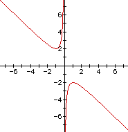
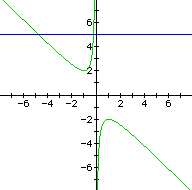
Consider the case when c = - 1 rather than + 1.
When c=-1, it is clear that the horizontal line, b=3 crosses the graph at two points. One root is always a positive x-value and one root is always a negative x-value. It also follows that any horizontal line will produce two intersections and thus two roots. Notice that these are the same observations we made when we graphed
Finally, let's explore the c value. We will set a= 1 and b=1 giving us the equation
Now, let's graph the equation for c=-3, -2, -1, 0, 1, 2, 3.
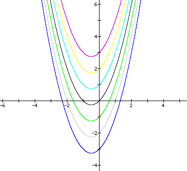
Notice that c shifts the graph
up and down c units. The parabola also passes through the c value on the y-axis. Exploring the roots of
we see that when a=1, b=1, c<0 the equation has one positive real root and one negative real root. When c=0, the equation has one 0 root and one negative real root. We will explore 0< c <1 to determine roots.
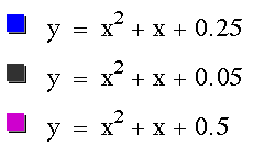
As you can see, the x-axis is tangent to our equation when c=0.25. Thus, when 0< c <0.25 our equation has two negative real roots, when c=0.25, our equation has one negative root, and when c>0.25 our equation has no real roots.
Remember that if you change the values of a and b the roots will differ as well.
In the following example the equation
is considered. If the equation is graphed in the xc plane,
it is easy to see that the curve will be a parabola. For each
value of c considered, its graph will be a line crossing the parabola
in 0, 1, or 2 points -- the intersections being at the roots of
the original equation at that value of c. In the graph below,
the graph of c = 1 is shown. The equation
will have two negative roots -- approximately -0.2 and -4.8.
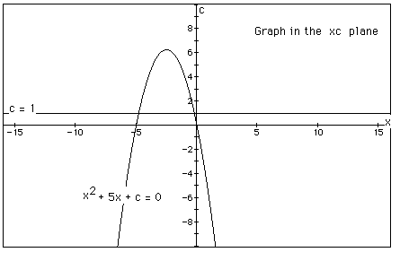
At c=6.25 the equation will have only 1 real root. For c >
6.25 the equation will have no real roots. For 0 < c < 6.25,
the equation will have two negative roots. When c = 0, the equation
will have one negative root and one 0 root. When c < 0, the
equation will have one negative root and one positive root.
Return to EMAT 6680 Home Page