

In this investigation, an attempt will be made to model a "cooling function" for a set of data. The experiment is fairly simple. A cup of water is brought to boil and the temperature is measured. The temperature is then measure each minute for the next 30 minutes. We will attempt to model a function to show the data and to predict some temperatures at a later time. We will also be using percent of error mathematics to show the model is adequate under the given circumstances.
| Time | Temperature |
| 0 | 212 |
| 1 | 205 |
| 2 | 201 |
| 3 | 193 |
| 4 | 189 |
| 5 | 184 |
| 6 | 181 |
| 7 | 178 |
| 8 | 172 |
| 9 | 170 |
| 10 | 167 |
| 11 | 163 |
| 12 | 161 |
| 13 | 159 |
| 14 | 155 |
| 15 | 153 |
| 16 | 152 |
| 17 | 150 |
| 18 | 149 |
| 19 | 147 |
| 20 | 145 |
| 21 | 143 |
| 22 | 141 |
| 23 | 140 |
| 24 | 139 |
| 25 | 137 |
| 26 | 135 |
| 27 | 133 |
| 28 | 132 |
| 29 | 131 |
| 30 | 130 |
On a scatter-plot the data is as:
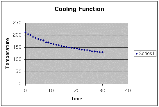
Upon observation a linear function (C(x) = mt + b) will not be an accurate description of the data. Also a quadratic will not suffice. It appears to need a exponential equation. We will attempt to model this data under the general form:
By the data when t = 0, C(0) = 212. By simple algebra:
Therefore we can observe our partial model as:
Clearly we must attempt to find a suitable p for the situation. There are an infinite values we can consider but let's first look at an algebraic attempt. Let's use another point on the curve, (t , C(t)) = (15 , 153). Note, p has been rounded to the nearest ten-thousandths.

Using identical algebra other p values for different (t , C(t)).
| Time | Temperature | P |
| 0 | 212 | |
| 1 | 205 | -0.0335762955336043 |
| 2 | 201 | -0.0266406833064684 |
| 3 | 193 | -0.031298695255709 |
| 4 | 189 | -0.0287098149030925 |
| 5 | 184 | -0.0283301034126054 |
| 6 | 181 | -0.0263482072343645 |
| 7 | 178 | -0.024971817768561 |
| 8 | 172 | -0.0261364747323199 |
| 9 | 170 | -0.0245319819579723 |
| 10 | 167 | -0.0238592462255257 |
| 11 | 163 | -0.0238941885332046 |
| 12 | 161 | -0.0229318258072958 |
| 13 | 159 | -0.0221293901885985 |
| 14 | 155 | -0.0223686541251976 |
| 15 | 153 | -0.0217432235519718 |
| 16 | 152 | -0.0207941096141085 |
| 17 | 150 | -0.0203500576809269 |
| 18 | 149 | -0.0195911093736974 |
| 19 | 147 | -0.0192712467312251 |
| 20 | 145 | -0.0189926266125719 |
| 21 | 143 | -0.0187496021148621 |
| 22 | 141 | -0.0185375629224475 |
| 23 | 140 | -0.0180410370462047 |
| 24 | 139 | -0.0175880142308884 |
| 25 | 137 | -0.0174642139537555 |
| 26 | 135 | -0.0173581344705224 |
| 27 | 133 | -0.0172680424611207 |
| 28 | 132 | -0.0169208697173443 |
| 29 | 131 | -0.0165996190162366 |
| 30 | 130 | -0.016301727473881 |
Looking over the possible values for p under our given model, the values vary more than expected. Let's look at the p-value for (15 , 153) which equals -0.0217. Therefore our equation would be:
When we plot the original data with our modeled function we obtain this graph.
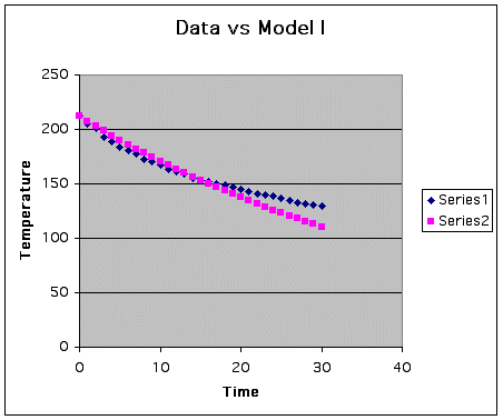
Where the blue curve is the data and the pink curve is the modeled.
Clearly not a bad start but not good enough. There is no reason to look at percent of error since it seems as if we are falling further and further away as the time gets closer to 30 and most likely above.
Let's adjust our general equation to, hopefully, flatten out our curve. Our new equation will take into account that the water will only cool to room temperature. We will assume that the room temperature is 72. What we are trying to get is that our equation will limit at 72 when t approaches infinity. To do this we must have a general equation as followed:
To find the values of our three parameters for this function we need to start with satisfying a and d. If we want to let the equation to limit at 72 as t approaches infinity we need to understand that when t approaches infinity the first part of our equation will approach zero. Clearly that would mean the d = 72. To find a will use our initial point (0, 212)
Now our equation is taking shape:
We then can use a data point to solve for a potential p to get some sort of idea where we need to be as far as picking a p-value. Like above it will require natural logs to solve. Let's use the final point (30 , 130)

Our second modeled equation will look as so:
If we plot our new model (Model II) vs the original data we have this graph.
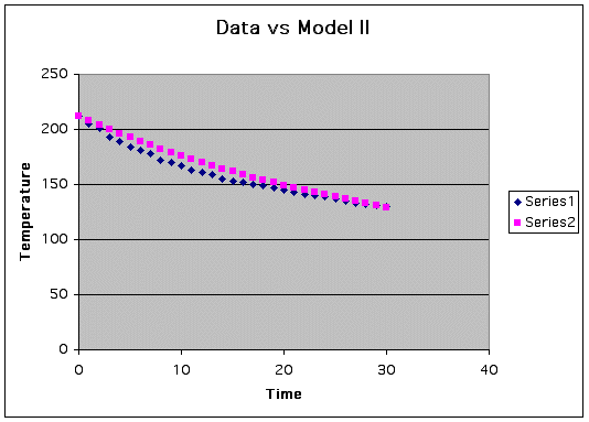
Clearly we have improved but still lacks enough visual evidence to due percent of error test. We will use the same general equation as we did in Model II but we will use a different (t , C(t)) to calculate p.
Model IIb Let's use (15, 153) to solve for p as we did above and will obtain the following equation for out cooling.
Graph vs original data:
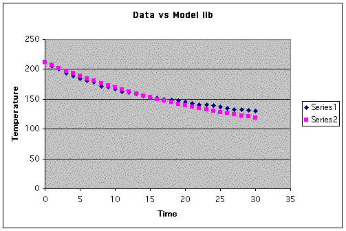
We seem to model the first 15 points fairly well but seem to fall off at a higher rate at t = 25 and above. The percent of error for this model is 31.29%. Far above a desirable number.
Let's generate another p for the same general equation and use the point (20, 145) which would give us the equation:
with graph:
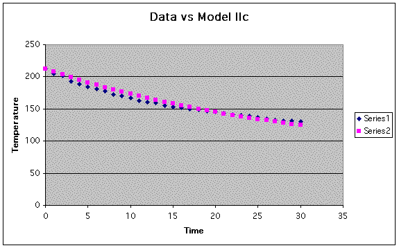
By using a higher value of t we seem to model the later end of the data better than the earlier end. Though it looks decent the percent of error is 19.85. Back to the drawing board.
NOTE TO READER:
Since it has not been discussed the percent of error is found by squaring the differences of the temperatures for each time, summing the squares, and dividing by the number of data points. Which in this case is 31.
As you can see by a decreasing p from -0.03648 to -0.03256 we have decreased the percent of error. Let's try another decreasing of p. Say to -0.032.
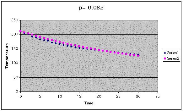
Clearly the error has grown. I then decided that we need not worry about the limiting parameter of d = 72. Numerous attempt were made and the following cooling function came about, with graph and percent of error.
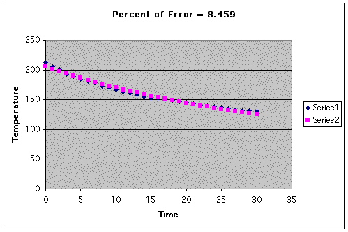
The curve was approaching the intended target but since a goal for my percent or error was around less than 1.5, I decided to switch the magnitude of the "a" and "d" values. That is I made a + d = 212 but made d > a. After many painstaking attempts here is my final model for the data.
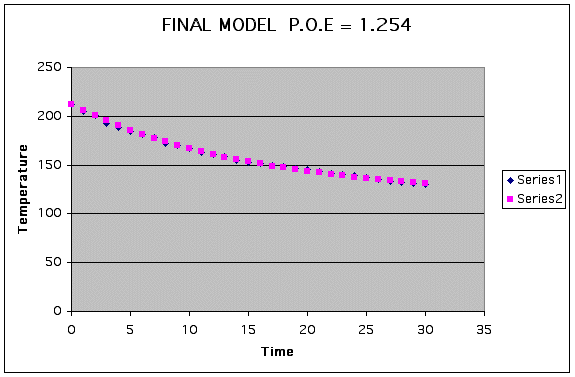
I would like to say that there was an easy process to finding this model but it mainly took hours of changing parameters. Too see the data chart for this model, including calculation of percent of error: CLICK HERE
We can use this model to predict the temperature outside of the range of times during the experiment.
For example:
1. Temperature after 45 minutes?
2. Temperature after 60 minutes?
3. Temperature after 300 minutes?
The major problem with the model is that the limiting factor of 118.3 will mean that the function will limit out there but for purposes of modeling the given data the function works nicely.
If you have a different model you would like to share with me please email it to me on my web page. I must admit this was the most frustrating of the twelve write-ups I have attempted, merely because of the trial and error it seemed to go through. It is worth noting that this write-up has opened my eyes as to the possibilities that spreadsheets have in mathematics. I have enjoyed the challenge and will definitely use it in my classes.
BFM