
The Department of Mathematics
Education
William Daly
EMAT6680
Write Up #10
Summer 03
Lissajous
Patterns at the Dawn of the Technological Revolution
The Lissajous pattern or Lissajous figure is named for the French mathematician Jules Antoine Lissajous[1]. Lissajous’ work in the nineteenth century
centered around the study of vibrating objects and wave phenomena. A method Lissajous used to study
vibration was to reflect light from a mirror attached to the vibrating
object. To study the relationship
between two vibrating objects, a mirror was attached to a tuning fork. Light was reflected from this mirror. The reflected beam was then reflected from a
second mirror attached to another vibrating tuning fork at a right angle to the
first tuning fork. After the second
reflection the beam of light was projected onto a screen, such that when the tuning forks were made to
vibrate a pattern developed that told a story about the relationship between
the two vibrating objects.
Fast forward to pre-modern electronic instrumentation. One of the earliest instruments, of great value to this day, is the oscilloscope invented at the beginning of the twentieth century. Modern instruments of various types, with high speed digital signal processing, are capable of extracting real time information from signals of interest. However, prior to the availability of such instruments, the oscilloscope was the mainstay electronic instrument to investigate electronic signals representing diverse parameters, from communications devices, musical instruments, parameters of mechanical systems to wide variety of other applications. The way the oscilloscope works is that a beam of electrons is project onto an fluorescent screen, just as in your television set or computer monitor. This beam is scanned across the screen linearly with time. The oscillating electronic signal in question is amplified and used to deflect the beam vertically. The result is an amplitude versus time display of the signal. For a simple x=sin ωt, the oscilloscope display would look similar to Figure 1.
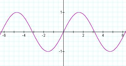
Figure 1
The horizontal axis is calibrated to time and the vertical
axis is calibrated to voltage, which can be made to represent a wide variety of
physical phenomena.
So what has all of this to do with the Lissajous figure? It turns out that to study the relationship between two signals, at least prior to the advent of today’s arsenal of advanced instruments, was quite difficult. To solve this problem, it was realized that Lissajous’ work may be of some value. Taking advantage of this, it was reasoned that the horizontal axis does not necessarily have to be a linear scan relative to time. It should be possible to have the horizontal axis be related to the amplitude of one signal, and the vertical axis be related to the amplitude of a second signal. While it is implicit that both of these signals vary with linearly time as they are trace out the display, a representation of time is not anywhere to be found on the display. The display is simply one signal amplitude (on the x axis) compared to another, possibly unrelated, signal amplitude (on the y axis). These signals may then be expressed as a parametric equation:
x=A1sin(ω1t)
y=A2sin(ω2t+θ)
Note that the second equation has a phase term “θ”, absent from the first equation. The reason for this is that we are free to choose any reference point in time, which is most convenient to be θ=0 for the first equation. So it is seen that θ is just a relative delay between the two functions. The addition of the phase term only makes sense if the two functions are harmonically related; for if they are not, the pattern of one function continually changes as shown in Figure 2 below. Note that on an actual oscilloscope display, the persistence of the trace is short lived so the result would be a continuously changing pattern. In the graphs we create, the persistence of the plotted points is as long as we choose to make it (by increasing the upper value of t). For all other graphs in this paper, the signals are harmonically related, so the pattern the repeats every 2π. But in the cases shown below, an approximation of the irrational number e is used as the relationship between the two signals. The number e was chosen for no other reason to cause the two signals in these traces to not be harmonically related.
Figure 2
Now lets explore how the Lissajous figure could aid one with only an oscilloscope to discover relationships between two signals. For each of the remaining graphs, the frequencies are harmonically related, that is the term multiplying “t” is a rational number. Therefore, the graph is a repeating function for some multiple of 2π. Let use begin with the case where the frequencies ω1 and ω2 are identical, and θ=0. Figure 3 shows the pattern is what would be seen on an oscilloscope display.
Figure 3
While this graph appears to be uninteresting, it does contain a great deal of information about the two signals. Note that at every time t, each x value is identical to each y value. Therefore, the two signals form the Lissajous figure of a straight line between (-1,-1) and (1,1). One can conclude from this that the two signals are of the same amplitude and phase (or delay).
Now modify the relationship a bit. Let us add a delay, or phase shift, to the second signal by leaving the amplitudes and frequencies the same and adding a phase of π/2 to the second signal. It should be recognized that this is the same as the cosine function:
In this case, the amplitude and frequency are still identical, both oscillate between –1 and +1, but do so 90˚ (π/2 radians) out of phase with each other. So this is an example of the an initial application of the Lissajous figure to determine that phase relationship between two signals. Click on the Figure 4 to see a dynamic display as the second function’s phase moves through a full cycle from 0 through 2π relative to the first function. Notice that when the two are exactly out of phase (180˚), the figure is a line from (-1,1) to (1,-1). Since the amplitude is unity, the pattern never ventures outside the unit square.
Can the Lissajous figure tell more than just phase? Look at the case where, the frequency and phase are the same, but the amplitudes differ. How would you expect this to alter the pattern. If one amplitude is twice the other, it would seem like an elliptical pattern would be the expected outcome. This is confirmed by the following pattern. Click on Figure 5 to observe varying relative amplitudes. The first amplitude is fixed; the second amplitude is varied between relative values of ½ to twice the first function.
Notice that the diagonal elliptical figure represented a difference in phase between the two functions, whereas in this case an elliptical pattern along the x or y axis indicates a difference in amplitude. Of course the locus of points is no longer restricted to the unit square since the amplitude of the second function is up to “2” as seen in the animation.
The Lissajous figure can also provide information about the relative frequency of the two functions. Two cases are provided that show the one frequency 3 times the first and then a case of one frequency 5/3 the first. In both cases, this pattern repeats every n·2π, where in is an integer because of the rational relationship between the frequencies.
Although the frequencies of either signal can not be extracted from these figures, the two graphs demonstrate that the Lissajous figure reveals information about the relationship between the frequencies of two signals. In the first graph, where the second signal is triple the frequency of the first, note that for every excursion over the signal period in the x direction, the signal in the y direction incurs 3 cycles. In the second case, for every 3 excursions over the signal period in the x direction, the signal in the y direction incurs 5 cycles. From viewing the Lissajous figure, the relationship between the signal frequencies can easily be counted.
Click on Figure 6 for 3x the frequency to see that amplitude information is obtainable from even these more complex figures. Also phase information is still available from the complex patterns, seen by clicking on Figure 7 for 5/3 x the frequency. In these cases, the degenerate figure (similar to the linear graph shown above) for which phase information cannot be seen is no longer a straight line. The degenerate cases occur at increments of (2n-1)·(π / 12), for n=1, 2, 3, …
To conclude, it can be seen that the mathematical relationship of two parametric equations can be exploited to extract information from real world situations. In the case of Lissajous figures, 19th century mathematics, demonstrated at that time using tuning forks and mirrors, played an important role in development and use of electronic equipment in the 20th century. Prior to the advent of high speed digital test equipment, technicians, engineers and scientist we were capable of extracting a wealth of information about the relationship of two signals, from many branches of science and engineering, by displaying a parametric form of signals on cathode ray tube.