
The Department of Mathematics
Education
William
Daly
EMAT6680
Write Up #12
Summer 03
Cooling
a Cup of Water
A
simple activity such as cooling a cup of water offers several opportunities to
explore mathematics. In this
investigation, the following mathematical activities and concepts are applied:
·
theoretical
principles modeled by mathematical expressions
·
expressing
empirical results in graphical form
·
fitting
theoretical predictions to measured data
·
altering
either the actual system or the model to better explain and fit the theory
·
comparing
the quality of the theoretical prediction with measure data
An
expression for the cooling of a cup of water is developed from basic
thermodynamic principles. This theory
is tested against a simple system, a cooling cup of water. In this exploration an Excel spreadsheet was
used to graph the empirical results and the theoretical prediction. The actual data and the mathematical
representation of the temperature of a cooling of an 8 ounce cup of boiling
water is graphed versus time. At t=0,
the heat was removed from the water and the temperature of the water was
measured at 1 minute intervals. Room
ambient temperature was monitored at ½ minute intervals to validate the
assumption that there was no significant time dependence in the room ambient
temperature. As will be seen, the match
between the predicted and actually values suggests there is something missing
in the model A conjecture was made as
to the cause of this disparity and the system was altered to minimize the
conjectured confounding variable. This
resulted in a substantially better match between actual and predicted
behavior. A method is proposed of
comparing these two systems versus the model.
Development of the Mathematical Model of the Theoretical Principle
This
exploration discusses a comparison the empirical results of cooling a cup of
boiling water with what would be predicted from the first law of thermodynamics[1]. The first law is expressed as a rate
equation
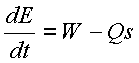
The
meaning of this equation is quite straight forward. It states that the rate
of change of energy in a system (dE/dt) is equal to the work, W, done on the
system or power entering the system, minus heat transfer rate Qs out of the
system.
In our experiment, at t=0, we assume that all
of the energy has been imparted to the system.
Therefore we set W=0 and this equation becomes:
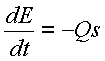
This
equation is very intuitive in that it simply states that the rate of change of
energy in the system is equal to the heat transfer rate. What is not immediately apparent though is
the detailed characteristics of the system, such as the heat capacity of the
liquid and the insulating, or transfer rate, characteristics of the
container. So at this point, it is
necessary to realize that the energy of the system is directly related to
temperature elevation or change and that the heat transfer rate can also be
measure in terms of a temperature difference over time. Therefore, this equation can be written in
terms of a temperature difference, T, versus time:
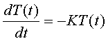
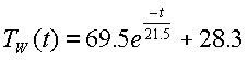
where
K is a constant, which will be empirically derived for the purposes of this
discussion. This simple differential
equation has the solution:
![]()
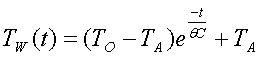
At
this time, it is convenient to impart physical meaning to the constants used in
this solution. Also note that T(t) was
defined as a temperature difference, so that the actual water temperature is
this temperature difference above an essentially time independent ambient
temperature: Then the water temperature
Tw can be expressed as:
![]()
There
are three characteristics of the system wrapped up in the constants A
and K. The constant A is related
to the initial temperature rise over the ambient temperature. Therefore, A=TO-TA. The constant K is related to the heat
capacity of the system and to the insulating characteristics. So call the insulating characteristics a
thermal resistance, q, and the heat capacity of the water C. Since the greater the insulation, or thermal resistance, and the
greater the heat capacity, the slower we would expect the temperature to
change, these constants are inversely proportional to K, thus:
Now
that a general expression for the water temperature has been developed, do a
quick sanity check on how this equation behaves. At t=0, the exponential is unity, and:
![]()
This
makes sense, since TO is just the initial temperature of the
boiling water (TO is approximately 100°C).
As
t →∞, the exponential approaches zero, and TW(∞)→TA,
the room ambient temperature, as we would expect.
Now
that we have what seems like a good candidate to describe the water temperature
as a function of time, the only unknown is the product of thermal capacity and
thermal resistance. Selecting a first
cut at this value ought be a simple matter by noting that at t=q•C, the exponential term has
an exponent of –1. Since e-1
has a value of about 37%, we can easily find the value of K by noting value of
t at which TW(t) has
change by about 63%. So this is a good
departure point to turn our attention to the empirical data.
Expressing Empirical Results in Graphical Form
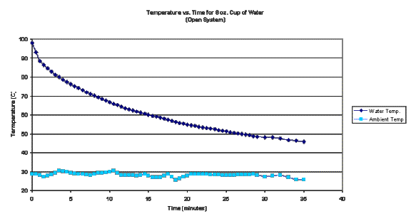
The
8 ounce cup of water was brought to boiling and at t=0 left to cool. The water temperature was taken at 1 minute
intervals and the ambient temperature was taken at ½ minute intervals. For the purposes of graphing both results,
both the water temperature and ambient temperature were linearly interpolated
to ½ minute intervals.
The
average ambient temperature was 28.3°C, with a standard deviation of 1°C. Since the standard deviation was less than
2% of the total temperature excursion, the ambient temperature is deemed to be
constant.
The
following is a graph of the data over a 30 minute period.
Fitting Theoretical Predictions to Measured Data
A
useful point in the data to notice is the time at which e is raised to the –1
power. This time, called the time
constant, occurs when the temperature has changed to about 37% of its final
value. Note that at about 21.5 minutes,
the water temperature change from 97.8°C to 54°C, which is 63% of the full
excursion to room ambient.
At
this point we have enough information from the empirical data to fill in the
constants for our equation for TW(t). A=TO-TA = 97.8°C - 28.3°C =
69.5°C; this is the difference between the starting temperature and the
final temperature, which is the average value at ambient. q•C = 21.5 minutes. So our equation to predict the water
temperature is
A
graph of the predicted temperature overlaying the data is shown below:
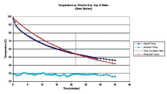
The
equation used to predict temperature is a moderate fit to the actual data, but
there is obviously something missing in modeling the system. The t=0 and t=21.5 (recall t is where e is raised to the
–1 power) the fit is perfect. This is
obvious since these are the points used to construct the functional
representation of temperature. Away
from these points there is apparently an excessively rapid cooling, compared to
the prediction, followed by a slowing in the cooling. If we have faith in the theory developed to describe the cooling
process, some reflection on the method of executing this experiment suggests
that the rapid cooling may due to a cooling mechanism beyond conduction through
an insulator. The most obvious of these
is the process of evaporation. Because
of this, this trial is dubbed an “open system”. The apparent slowing in the cooling process is possibly an
artifact of having chosen an incorrect value for the time constant.
Altering Either the System or the Model
Having proposed a
possible explanation for the discrepancy in the theoretical versus the data, we
have a choice of how to explore this.
This choice depends upon our objectives.
On the one hand, if
the objective is to describe our original system, we need to note that
suspecting evaporation as a contributor to the discrepancy calls into question
an earlier assumption. That assumption
is that the system is described by a change in energy merely by heat transfer
and that there is no net work done on the system. This can only be true if there is no significant change in the
mass of the system If evaporation is a contributor,
then there is work done on the system as a result of water vapor leaving the
system, taking heat with it. This is in
contrast to heat simply being conducted to the surrounding air through the
walls of the container. Using this as
an objective would require rewriting the original rate equation and finding the
associated solution. This requires
“fixing” the theory.
On the other hand
if our objective is to describe a system whose primary method of heat transfer
is through conduction, it is reasonable to suppose that the theory is still
valid, but the actual model is flawed.
In this case, “fixing” the system is required.
To execute a second trial, this second objective is used. So the we can suppose that the solution to the original rate equation applies, but that we must somehow change the system we perform the experiment on. To test this modification, the experiment was repeated as a “closed system”, which was done by simply covering the cup with a ceramic plate. Note that this system was nearly closed, since there was a small gap, approximately 1mm, between the plate and the cup for the temperature probe to pass through. Repeat of the experiment using a closed system resulted in the following graph.
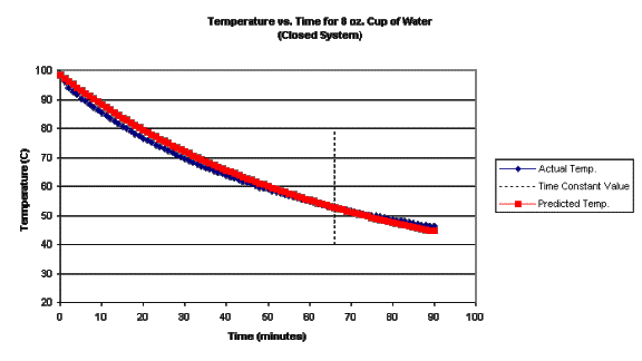
From
two characteristics of the graph for the closed system trial, it apparent that
evaporation is indeed a significant part of the cooling process in the open
system. First, for a similar
temperature range, the closed system trial took over twice as long. The implication here is that evaporation was
the dominant cooling process in the open system which was minimized to a very
great extent in the closed system. The
second point to notice is that the agreement between actual data the
theoretical prediction is significantly better in the closed system.
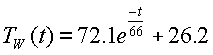
The ambient temperature at the beginning of the experiment was 26.2°C. In the closed system, the heat capacity did not change. But the thermal resistance and transfer rate. Whereas evaporation appears to have been the dominant source of cooling in the open system, now this mode of energy change has been made negligible. Therefore, using the method outlined above, a new value of 66 seconds was chosen for the time constant where the temperature changed by 63% of its full range. Then the equation used to predict the temperature in the graph for the close system is:
The
statement that the experimental and theoretical agreement for the closed system
is much better than for the open system is a result of visual inspection of the
two graphs. To quantify this statement,
the idea of MSE (mean square error) is used to quantitatively compare the two
trials.
Comparing the Quality of the Theoretical Prediction With Measured Data for Open and Closed Systems
The statement was made above that the agreement between experimental and theoretical results was much better for the second trial. While this seems obvious from the graphs, there ought to be a way of quantifying how much better the prediction is. One possible method for expressing this is look at what is know as the RMS (root mean square) error.
In general terms for a discrete series of data
point, this error is expressed as:
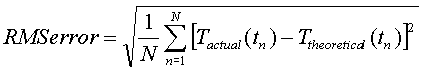
Evaluating this expression in Excel is a very simple matter. A column is added next to each of the data point with a formula that is the square of the difference between the experimental and theoretical values. This column is summed and then divided by the total number of data points. Finally the square root of this result is taken. Doing so results in the following comparison to the closed and open systems:
Open system RMSerror = 4.1°C
Closed system RMSerror =
1.8°C
While it is convenient to get a single number
representation as to how good our results are, why go through all of the
trouble of calculating the error in this way.
Although the RMS concept has an actual physical meaning in many branches
of science, part of its utility here can be seen from a couple of observations. One may wonder why we do not just look at an
average error. The problem with using
an average is apparent if we consider say a very large mismatch between actual
and predicted results, but the error is, say, in the shape of a large amplitude
sine function. This would be a horrible
match, but still the average error would be zero, a very deceiving
representation of the error. Notice
that the difference in calculating RMSerror is the squaring of the difference
between actual and theoretical. This
eliminates the deception inherent in an average comparison because all square
values are positive. These squared
values are then summed, and in a sense the average is taken by dividing by the
number of data points. This result is a
better comparison between different trials, but to relate it back to a physical
meaning, temperature in this case, the square root must be taken of this final
value. So in the calculation of the RMS
error of the two experiments, there is a single digit representation of how the
data fits the theory, about 4.1°C for the open system, whereas, the overall
difference between actual and theoretical is about 1.8°C.