
Janet Kaplan
Cooling Water Function
__________________________________________________________________________________________________________________
In this investigation we
are given data involving the temperature of boiling water as it cools,
ultimately, to room temperature. Starting at 212 degrees Fahrenheit, the
temperature of the water is taken every minute for 30 minutes.
The data is graphed below,
with the independent variable as time in minutes and the dependent variable as
temperature.
Given this data, how can we
predict what the water's temperature will be in 45 minutes, or 60 minutes, or
even 300 minutes?
____________________________________________________________________________________________________
Our first task will be to
determine specifically what the cooling function is. This is real life,
however, and chances are the data will not fit neatly into a perfectly smooth
line or curve. We must, therefore, determine a best-fit curve for our
data.
How do we begin to do this?
Take a look at the shape of
the curve. What type of function best models our data? It doesn't look linear,
as it is not a straight line. It's not a quadratic function, for it has no
resemblance to a parabola. Nor is it any higher level polynomial, again because
it has no similarity to a cubic or higher degree equation.
It's clearly not a
trigonometric function, for there is no periodicity. There are a few other
families of functions that also do not apply. But what our data does resemble
is an exponential function. More specifically, a decreasing
exponential function, often known as a decay
curve.
Notice that it starts off
at 212 degrees and decreases fairly rapidly at first. As time moves on, the
water temperature is still decreasing, but at a somewhat slower rate. Although
it's hard to see on the graph, with each minute the reduction in temperature
progresses at a slower rate. At 30 minutes it is down to 130 degrees. We can
surmise that the water will continue to cool, and that ultimately it will come
to rest at room temperature (let's say 70 degrees).
So we will begin by trying
to find the best-fit exponential function for our data.
There's a catch, however.
Exponential functions increase or decrease without bounds (to infinity). But
experience tells us that the water will maintain the temperature of the air
around it indefinitely, not decrease to absolute zero. So we will need to modify
our model to incorporate this fact.
____________________________________________________________________________________________________
At this point we can
approach the problem from one of two ways. We can use a spreadsheet
application, like Excel, to show us the results of otherwise time-consuming
calculations quickly and easily. Or we can graph a general exponential model
using Graphing Calculator software. Often it is helpful to use both avenues
simultaneously.
The general form of a
decreasing exponential function is y = ae-bx, where a is
the starting value, e is the natural base, (-b) is the rate of decrease, and x
is the time in minutes. In our example, a will be the starting temperature, and
(-b) will be the cooling rate.
Exponential functions
increase or decrease by the same multiplicative factor each time period. That
is, we multiply or divide by b for each unit change in x. My first model is
saying that starting at 212 degrees, the temperature
will decrease from the previous temperature by e -0.02 every minute.
Here I have used Excel to list
the actual data along with temperature calculations using My First Model, y=212e^-0.02x.
|
|
Actual |
|
|
y=212e^-0.02x |
|
|
|
|
|
|
|
|
|
|
Actual |
|
|
My First |
|
|
Minute |
Temp |
diff |
|
Model |
sq of diff |
|
0 |
212 |
0 |
|
212.00 |
0.00 |
|
1 |
205 |
7 |
|
207.80 |
7.85 |
|
2 |
201 |
4 |
|
203.69 |
7.22 |
|
3 |
193 |
8 |
|
199.65 |
44.28 |
|
4 |
189 |
4 |
|
195.70 |
44.90 |
|
5 |
184 |
5 |
|
191.83 |
61.24 |
|
6 |
181 |
3 |
|
188.03 |
49.38 |
|
7 |
178 |
3 |
|
184.30 |
39.74 |
|
8 |
172 |
6 |
|
180.65 |
74.90 |
|
9 |
170 |
2 |
|
177.08 |
50.09 |
|
10 |
167 |
3 |
|
173.57 |
43.18 |
|
11 |
163 |
4 |
|
170.13 |
50.89 |
|
12 |
161 |
2 |
|
166.77 |
33.24 |
|
13 |
159 |
2 |
|
163.46 |
19.92 |
|
14 |
155 |
4 |
|
160.23 |
27.31 |
|
15 |
153 |
2 |
|
157.05 |
16.43 |
|
16 |
152 |
1 |
|
153.94 |
3.78 |
|
17 |
150 |
2 |
|
150.90 |
0.80 |
|
18 |
149 |
1 |
|
147.91 |
1.19 |
|
19 |
147 |
2 |
|
144.98 |
4.09 |
|
20 |
145 |
2 |
|
142.11 |
8.36 |
|
21 |
143 |
2 |
|
139.29 |
13.73 |
|
22 |
141 |
2 |
|
136.54 |
19.93 |
|
23 |
140 |
1 |
|
133.83 |
38.04 |
|
24 |
139 |
1 |
|
131.18 |
61.12 |
|
25 |
137 |
2 |
|
128.58 |
70.82 |
|
26 |
135 |
2 |
|
126.04 |
80.31 |
|
27 |
133 |
2 |
|
123.54 |
89.44 |
|
28 |
132 |
1 |
|
121.10 |
118.89 |
|
29 |
131 |
1 |
|
118.70 |
151.33 |
|
30 |
130 |
1 |
|
116.35 |
186.37 |
|
|
|
|
|
|
|
|
|
avg diff |
2.73 |
|
|
47.29 |
I have also calculated the deviation
between my model and the actual data using the least squares method. 47.29
is higher than we would like; we want this value to be
as close to zero as possible.
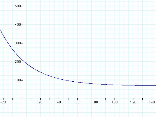
Here is a graph of the
data, comparing the actual data to my first model. How close did I come?
Notice that my model decreases too gradually at first,
and then too quickly later on. I’ll need to do some refinement.
This is also a good time to
think about including the limiting temperature in my model. How do I build this
in?
Newton’s Law of Cooling
states that the final temperature of an object that is warmer than the air
around it can be determined by the formula Tf = Tr + (T0 – Tr)e-rt, where Tf is the final temperature after t minutes, Tr is the temperature of the surrounding air, T0
is the original temperature of the object, and r is the rate at which the
object is cooling.
We can state the same thing
this way: y = c + ae-bx ,
where c is the minimum temperature (70), a represents the range of temperatures
in the function (212-70 or 142), (-b) is the cooling rate, and x is the time in
minutes.
We’ll use Graphing
Calculator now to graph this function. CLICK HERE to
manipulate the function yourself.
y = 70 + 142e-0.325x
You may wonder how I knew
what value of b to use. Nothing beats trial and error, and nothing beats technology’s
capacity to help in this matter. Starting with b = -.1, I just kept using
different values in Graphing Calculator until I came as close as comfortable to
the curve I was looking for. I then entered my figures into Excel and
calculated the deviation again using the least squares method.
|
|
Actual |
|
y=70 +
142e^-.0325x |
||
|
|
|
|
|
|
|
|
|
Actual |
|
GCF |
|
|
|
Minute |
Temp |
|
(b=-.0325) |
sq of
diff |
|
|
0 |
212 |
|
212.00 |
0.00 |
|
|
1 |
205 |
|
|
|
|
|
2 |
201 |
|
|
|
|
|
3 |
193 |
|
|
|
|
|
4 |
189 |
|
|
|
|
|
5 |
184 |
|
190.70 |
44.89 |
|
|
6 |
181 |
|
|
|
|
|
7 |
178 |
|
|
|
|
|
8 |
172 |
|
|
|
|
|
9 |
170 |
|
|
|
|
|
10 |
167 |
|
172.56 |
30.91 |
|
|
11 |
163 |
|
|
|
|
|
12 |
161 |
|
|
|
|
|
13 |
159 |
|
|
|
|
|
14 |
155 |
|
|
|
|
|
15 |
153 |
|
157.21 |
17.72 |
|
|
16 |
152 |
|
|
|
|
|
17 |
150 |
|
|
|
|
|
18 |
149 |
|
|
|
|
|
19 |
147 |
|
|
|
|
|
20 |
145 |
|
144.13 |
0.76 |
|
|
21 |
143 |
|
|
|
|
|
22 |
141 |
|
|
|
|
|
23 |
140 |
|
|
|
|
|
24 |
139 |
|
|
|
|
|
25 |
137 |
|
133.01 |
15.92 |
|
|
26 |
135 |
|
|
|
|
|
27 |
133 |
|
|
|
|
|
28 |
132 |
|
|
|
|
|
29 |
131 |
|
|
|
|
|
30 |
130 |
|
123.56 |
41.47 |
|
|
|
|
|
|
|
|
|
|
avg diff |
|
|
25.28 |
|
At a deviation value of
25.28, I came very close to a function that models the actual cooling data.
I then use this model, y = 70 + 142e-0.325x, to predict the water
temperature at 45, 60 and 300 minutes. The values are, respectively,
45 minutes 102.90
degrees
60 minutes 90.20 degrees
300 minutes
70.01 degrees
RETURN
to Janet’s Home page