Assignment 10: Parametric Equations
Definitions
Key Points:
A parametric curve in the plane is a pair of functions
![]()
where the two continuous functions
define ordered pairs (x,y). The two equations
are usually called the parametric equations of a curve. The extent of the curve
will depend on the range of t and your work with parametric equations
should pay close attention the range of t . In
many applications, we think of x and y "varying with time t " or the angle of rotation that some line
makes from an initial location.
Various graphing technology, such as the TI-81, TI-82, TI-83, TI-85, TI-86,
TI-89, TI- 92, Ohio State Grapher, xFunction, Theorist, Graphing Calculator 3.2, and Derive,
can be readily used with parametric equations. Try Graphing Calculator 3.2
or xFunction for what is probably the
friendliest software.
Explorations
Click the Graphing Calculator File to run any of these problems.
1. Graph
![]()
How would you change the equations to explore other graphs?
-> where to start with a boundless question like that! Within the family of sin\ cos curves the most obvious places to start are the overall coefficients [acos(t), bcos(t)], the period (coefficient for t) and the squaring of various elements.
2. For various a and b, investigate
![]()
Very interesting if we just consider changing a (only the ratio between a and b matters anyway unless one is 0.
At a = 1 we have the circle as above.
0 > a <1 – series of interesting curves with distorted sinusoidal properties.
a = 0, a vertical line at x =1 from y = 1 to -1, as makes sense, but a very different form.
-1>= a < 0 : mirror of above curves, including a circle at a = -1 (just drawn in opposite direction)
1> a >2 series of shapes just like 0 to 1 but rotated 90 degrees along y axis.
a = 2 : parabola with vertex at (1,0) and facing –x direction
as 'a' gets larger it has 'nodes' at the integer values with even and odd values having distinct curve types. Even values generate parabolic curves, facing in + or – directions alternately, and with a number of 'humps' (foci) = a/2. Odd integers beginning with 1 form a closed set of curves with 'nodes' = 1.
Really a very interesting set of equations with remarkable variety of forms by just varying one parameter.
3. For various a and b, investigate
![]()
Very easy to visualize and not as interesting as 'a' and 'b' change only the 'amplitude' of the curve in the x or y direction. Ellipses are formed which squish to a line when one coefficient is 0.
4. Graph
Interpret. What would you change to explore and understand the graphs?
-> A circle – surprise - very intriguing to change the
range of t. a
range of -1 to 1 graphs the right side of a circle, with the – range plotting
the lower arc and the + the upper arc. Increasing
the range to
Changing the 2 value in the y equation makes elliptical curves of course, which opens the question of 'why is 2 a circle'. Suspect this may be because of factoring (1+x)^2 has a 2x coefficient. If we solve equations and get factors we'll get to bottom of this.
5. Graph several sets of curves for
![]()
for selected values of a, b, and k in an appropriate range for t. (Set a and b and then overlay graphs for several values of k. Repeat for new values of a and b.)
interesting is that when a = b and k = 1, it always goes through origin. 'origin' of line when t = 0 may be shifted to (a,b), but the equal proportions of t for x and y will always get a line through origin.
As expected, k determines the slope of the line. If the ratio of b/a = k, the line will go through the origin.
6. Graph
![]()
for some appropriate range for t. Interpret. Is there anything to vary to help understand the graph?
This is just a specific version of the graph in 5. The 'origin' point of the line for when t = 0 is at (1,-1). Intriguing that these parametric curves always have a point defined if they include a numeric value in the equation. As we adjust the range of t, we can see again the ration of the y/x coefficients of t determine the slope of the line. In this case it's 2/1 =2.
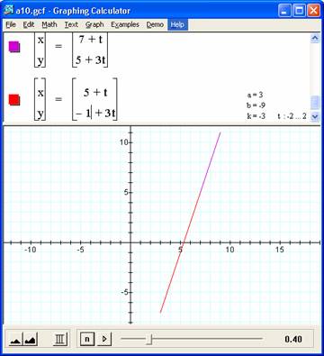
7. Write parametric equations of a line through (7, 5) with slope of 3.
Graph the line using your equations.
|
Easiest to see is when the 'zero point' for the line is at (7.5), as below X = 7+ t, Y = 5+3t. But any equation with an inclusive range of t and numeric values that are increased\decremented by values proportional to the t coefficients will work as well. For example, if we subtract from the (7,5) point the values of t = 2, we get an x= (7 - 2) and y =(5 -3(2), so the equations of: X = 5 + t, y = -1 + 3t works as long as the range of t includes t = 2. See the red graph that ends at point (7,5). |
|
8. Investigate
![]()
for different values of a and b. What is the curve when a < b? a = b? a > b?
-> Explored in 3 above. Very easy to visualize as 'a' and 'b' change only the 'amplitude' of the curve in the x or y direction. Ellipses are formed which squish to a line when one coefficient is 0.
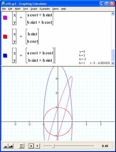
Describe fully. What is changed if the equations are
![]()
where h is any real number?
|
To help in this, lets graph the various components of the equation separately. In a way, we are adding a circle (hsint, hcost) to our original ellipse. Of interest is the impact of swapping the added components of the 'h circle' so our x has both cosine values and y both sin values. In this case it is easy to see that the original ellipse is expanded by the values of the h circle. This contributes back to our understanding of the primary equations of interest as graphed in pink. The 'off phase' aspects of adding a sin and cos together with differing amplitudes can be seen as the ellipse tilts on the axis. |
|
Investigate with graphs for small h (e.g. -3 < h < 3).
NOTE: These latter parametric equations
describe the locus of the vertex (x,y)
of a triangle with altitude h whose other two vertices are moved, one along the
x-axis and the other along the y-axis.
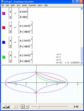
9. Investigate each of the following for
![]()
Describe each when a = b, a < b, and a > b.
|
x = a cos(t), y = b sin (t) · a = b : circle plain as simple · a < b : ellipse tall in y direction · a > b : ellipse tall in x direction x = a (cos(t))^2, y = b
(sin(t))^2 · a = b, a < b, a > b: intriguing – the Pythagorean Theorem kicks in. The squares get rid of all negative values so just in the first quadrant x = a (cos(t))^3, y = b
(sin(t))^3 · a = b : The (<0) aspect of sin and cos cause their squares to get increasingly small – causing the curves to get increasingly concave for larger exponents. Given the odd power, the original sign of the values is preserved once again, so in all quadrants. · For a < b and a > b. – stretches the curve in y or x direction respectively, as always For larger exponents, the pattern repeats, with the concavity of the curves getting more extreme. |
|
10. Consider
![]()
This equation would be difficult to graph with most
applications other that Graphing Calculator 3.2 .
Putting it in parametric form makes it possible to graph it with many other
applications (including the TI-81 or TI-82).
Let y = tx cross the curve at (0,0) and at P(x,y).
Then, substituting, (What is the basis of this magic? Need
to find out logic)
and so we have the parametric equations
Graph the curve using the parametric equations for a
suitable range of t.
Graph
![]()
using Graphing Calculator 2.1 or Algebra Xpresser for comparison.
Interesting that it graphs just the loop but not the arms.
11. Investigation. Consider the parametric equations
Graph these for
![]()
Describe fully. You may have to increase the range of t for the larger fractions.
-> cool shapes
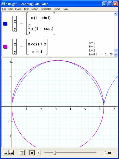
12. A cycloid is the locus of a point on a circle that rolls along a line. Write parametric equations for the cycloid and graph it. Consider also a GSP construction of the cycloid.
I should do the sketch in GSP but too lazy.
If we look at the circle as it rolls, we can probably model assuming a theta that represents this rolling 'wheel'. We have choices on how to orient the angle measure, but we know that we want the y value to go from 0 (at a theta of 0) to 2 * our radius R (at a theta of pi – as the wheel rotates one half revolution at that mark at the bottom of our tire is now at the top, and then down again.
A logical equation for y in this case is: vertical distance of centre - vertical component of rotating are = R – Rcos(T) where T = our angle theta in radians. This gives us a 0 at the
The x keeps getting bigger so it's a multiple of the R value and, just as for the y value, we need to correct for the oscillating horizontal component of the arm of our wheel.
X = RT - Rsin(theta)
So for any point P(x,y),
x = R(T- sinT) and y = R(1 - cosT),
where 0 <= T <= 2Pi
What's interesting is to see the difference in the semi circle and the cycloid. If we mess with the y coefficient in the cycloid equation and overlay a circle, we can see the shape is indeed different, but close.
|
|
|
|
|
|