Assignment 11: Polar Equations
Graphing Calculator
3.2 and xFunction are
suggested for these investigations. Subsitute
![]() for
t in these investigations. Some of them could be done with a TI-83 or similar.
for
t in these investigations. Some of them could be done with a TI-83 or similar.
Click the Graphing Calculator File to run any of these problems.
Key Points:
I really like my GSP scripts for animating the creation of these
basic curves for cos(2θ) s GSP script and cos(3θ) GSP script. Take a look see.
Also, these plots are fun looking:
1. Investigate
![]()
The base r=cos(kθ)
equation
|
The fundamental shape will come from the k coefficient of θ, so lets first vary that with a = 0
and b = 1. The others will have a
simple and predictable impact on the shape. K=0 yields a circle
centered at the origin of course, as the cos(0) is 1. K=1 – we get a
circle with radius .5 at center (.5,0) – Interesting because we would think
that as θ plots around the 2nd and 3rd quadrants
we would get a curve over there but the – cos value ( a – r value) is in
perfect phase with the θ value itself and the point reverses itself to
plot again back in the quadrant 4 for quadant 2 and quadrant 1 for quadrant
3. |
|
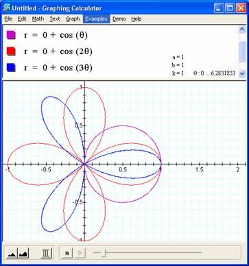
K=2. – The 'phase
cancellation' that occurs for k = 1 doesn't happen here so the 2 circles that
we would have expected there are intuitively doubled to a four leaf shape that
has leaves narrowed to ½ as wide as long (relative to the circle) because the
angle in increasing twice as fast. It's
instructive to trace the path of this curve to see what's going on:
See this GSP script to view this curve getting traced. It makes sense as we look at it but takes some thinking to see how the curve is traced as theta increases.
K=3. – See this GSP script to view this curve getting traced. This use of GSP is really nice because it makes it easy to see how the curve gets traced over twice for this odd multiple of theta, just as happened for k=1. GSP is useful because, while it's easy to trace in the head with k=1, it's hard to follow the construction for larger k values.
|
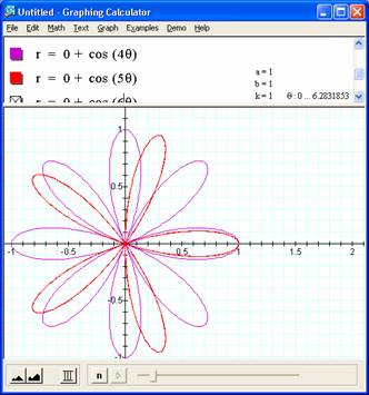
Postulate: This pattern leads us to speculate that odd multiples of theta (k) will generate overlapping curves and thus a number of leaves = k, and an even k will generate a number of 'leaves' = 2*k. Doing the additional graphs shows that this is indeed true. |
|
|
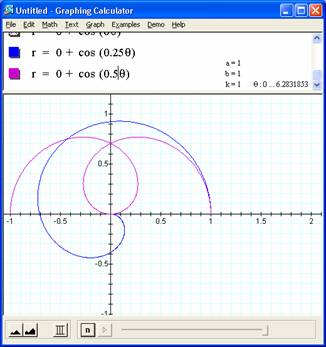
Fractional k values of .25 and .5 also generate interesting curves, especially the spiral formed by 'twisting' the base cosine traverse ( from 1 to 0 during the theta range of 0 to pi/2 ) all the way around the 2pi rotation. This spiral must has a name and interesting properties – for another day. |
|
Adding a 'b': r = bcos(kθ) equation
Not that spectacular really – just doubles the radius (size) of the graph as we would expect.
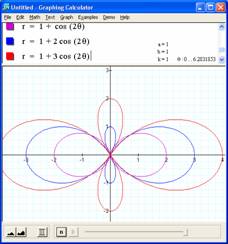
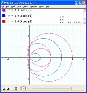
Adding a 'a': r = a+ bcos(kθ) equation
|
Adding a constant a to the base equation yields interesting curves. It is the addition of a circle around the origin (with some quadrant 2 & 3 plots) to our circle that spans quadrant 1 and 4 Note: Use the term quadrant loosely as this is polar coordinate system.
|
|
If cos( ) is replaced with sin( ) the above curves are simply rotated 90 deg (pi/2 rad) as we would expect.
2. Vary a, b, c and k
Subsitute ![]() for
t
for
t
The above graphs are
investigated thoroughly in 1. above excepting the last.
|
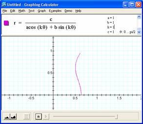
Strange behaviors
of an odd curve for parameter values as to the right. The curve reaches
up to a 'y value' of almost 3 with a range of θ: 0 – pi/2. Yet for a range of 0 – 10, the curve
reaches only 2.5 or so. Seems strange. For a θ of 0
I would expect r = 1/(1(cos(0) + 1 sin(0)) = 1 – but the graph shows a .63
value, dunno. |
|
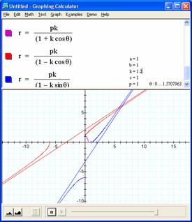
Note: The parameter k is called the "eccentricity" of these conics. It is usually called "e" but for many software programs e is a constant and can not be set as a variable.
For notes on a derivation of these formulas, click here.
An interesting set of curves as shown for the parameters below.
|
|
|
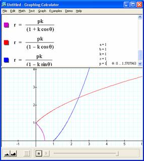
Varying p won't do anything really, but k has interesting changes. Makes me want to plot three dimensionally, as below
|
|
|
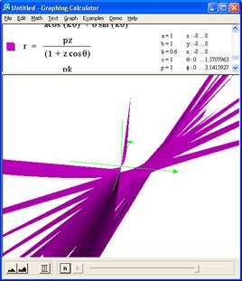
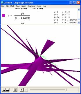
One of the strangest looking curves ever.
Subsitute ![]() for
t
for
t
Replace t by ![]() .
.
(Note: some of these graphs may become
more interesting -- or disasters -- when ![]() is
replaced by some f(
is
replaced by some f(![]() )
such as 2
)
such as 2![]() or 0.5
or 0.5![]() or 3
or 3![]() - 1 or . . .
- 1 or . . .
|
|
|
|
|
|