Assignment 3: Quadratic Equations
Some Different Ways
James W. Wilson and
Notes:
Revisions in red.
Click the Graphing Calculator File to run any of these problems.(program crashed & lost most so not all are in here)
It has now become a rather standard exercise, with available technology, to construct graphs to consider the equation
![]()
and to overlay several graphs for different values of a, b, or c as the other two are held constant.
![]()
The movement of the parabola for changing a, b, and c
Discussion of the dynamics of the coefficients and roots for:
![]()
is instructive. For example, if we set
![]()
for b = -3, -2, -1, 0, 1, 2, 3, and overlay the graphs, the following picture is obtained.
We can discuss the "movement" of a parabola as b is changed. The parabola always passes through the same point on the y-axis ( the point (0,1) with this equation). For b < -2 the parabola will intersect the x-axis in two points with positive x values (i.e. the original equation will have two real roots, both positive). For b = -2, the parabola is tangent to the x-axis and so the original equation has one real and positive root at the point of tangency. For -2 < b < 2, the parabola does not intersect the x-axis -- the original equation has no real roots. Similarly for b = 2 the parabola is tangent to the x-axis (one real negative root) and for b > 2, the parabola intersects the x-axis twice to show two negative real roots for each b.
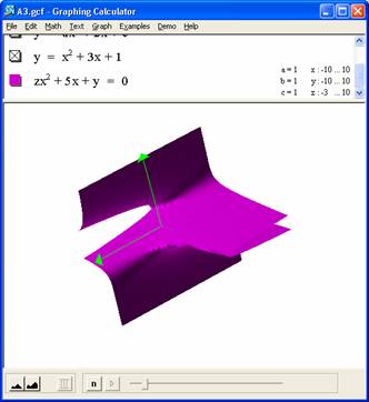
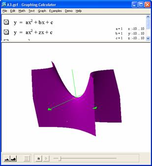
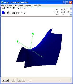
It's easy to visualize this in 3 dimensions, so let's do that first. If we graph using the z axis to represent b with x,y,z ranges from -10 to 10, we get the following:
|
|
|
From this we can see that as b (z on the graph) varies, the vertex of the
parabolic curve moves from below from a negative to positive y location, and
then back again. Also, the parabolas are
not symmetric about the y axis during this movement, as the preliminary graphs
suggested. This is difficult to see in
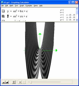
these 3-D shots, but note the visibility of the z axis in the 2nd
graph. The 2nd graph also
highlights an interesting property of the vertex of the xy
parabola as b (z) changes. It appears to
also form a parabola in the yz plane. To prove, lets use
algebra.
Algebraic support for visualization
A useful quadratic form for gaining understanding is:
y = a (x - k) ^2 + h.
In this form it is easy to see that the vertex of the
parabola will have a maximum y value at x = k when a < 0 or a minimum y
value at x = k when a > 0.
If we convert the general quadratic form y = ax^2 + bx + c into this format, we will be able to enhance our
analysis of this and other quadratic curves.
Using Algebra we know that the general quadratic can be converted to:
y = a (x + b/2a ) ^2 + (4ac – b^2) /4a
Which maps to the k and h form above, with:
-> k is -b/2a: Since the vertex will occur at x = k, in this general quadratic form the vertex occurs at x = -b/2a.
-> h is (4ac –b^2)/4a: So the y value of this vertex will be (4ac –b^2)/4a = c – b^2/4a
Dynamics of b for a simple example
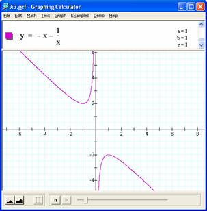
Let's investigate this for the simple form of the equation:
![]() .
.
Using the above equations, for [a=1, b, and c=1] we reduce to the vertex location (x,y) occurring at:
x = -b/2*1 = -b/2
y = 1– b^2/4*1 = 1-b^2/4
This provides support for our findings above related to vertex and roots of this equation around b = +/- 2.
Getting back to apparent movement of the vertex of the vertex as b (z) changes, we need to map this vertex in the yb plane (yz plane in the 3-D graphs above).
To find the curve of the vertex, we can solve for b in the b(x) relationship to get b = -x/2 and then substitute this into the y(b) equation to get the y(x), so
y(x) = 1-b^2/4 = 1-((-x / 2) ^2 ) /4 = 1 – x^2
so we’ve proved that the vertex of this curve follows the parabola y = 1 – x^2
General equation for the path of a vertex
|
Using the general equations for the vertex as above, we can solve for b and substitute to find a y(x) function. From above, the vertex for a general quadratic occurs at x = -b/2a, y = c – b^2/4a b(x) = -2ax, so y = c – ( (-2ax)^2 )/4a = c – 4a^2x^2/4a = c - and y = c – ax^2 |
|

Graphs in the xb plane.
|
Consider again the equation
To better mentally graph this relation in the xb plane we can solve for b(x) so we get b(x) = -(x^2 . We get the following graph. |
|
If we take any particular value of b, say b = 3, and overlay this equation on the graph we add a line parallel to the x-axis. If it intersects the curve in the xb plane the intersection points correspond to the roots of the original equation for that value of b. We have the following graph.
For each value of b we select, we get a horizontal line. It
is clear on a single graph that we get two negative real roots of the original
equation when b > 2, one negative real root when b = 2, no real roots for -2
< b < 2, One positive real root when b = -2, and two positive real roots
when b < -2.
Consider the case when c = - 1 rather than + 1.
Consider again the equation
![]()
|
If we consider the c = -1 case then we are evaluating the case X^2 + bx – 1 = 0 Again, to better mentally graph this relation in the xb plane we can solve for b(x) so we get b(x) = (1-x^2) /x = 1/x - x We get the following graph, where the red lines indicate this new hyperbolic curve. |
|
Using the same logic for reviewing a particular b value as a
horizontal line, we see that this equation has real roots for all b. If b is 0 we have the solution pair of +/-
1, which makes sense in the form x^2 + 0x -1=0 or (x
|
To easily get a visual of the impact of a varying c on this we can plot X^2 + yx + z = 0 This shows (easier when manipulating 3-D graph) that for c > 0 the range of null solutions expands to greater b values and as c < 0 it always has solutions per the hyperbolic curves above. It's easy to see that the saddle is not symmetric about the y axis but rather askew. In fact, it is readily seen that for c = 0 the solution set is of the form b = -x. |
|
Graphs in the xc
plane.
In the following example the equation
![]()
|
is considered. If the equation is graphed in the xc plane, it is easy to see that the curve will be a parabola. For each value of c considered, its graph will be a line crossing the parabola in 0, 1, or 2 points -- the intersections being at the roots of the original equation at that value of c. In the graph, the graph of c = 1 is shown. The equation
will have two negative roots -- approximately -0.2 and -4.8. |
|

There is one value of c where the equation will have only 1 real root -- at c = 6.25. For c > 6.25 the equation will have no real roots and for c < 6.25 the equation will have two roots, both negative for 0 < c < 6.25, one negative and one 0 when c = 0 and one negative and one positive when c < 0.
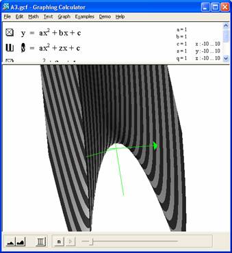
Again, because it's so easy and fun to do, lets allow b to vary as the x variable and plot for z from -3 to 10 to more easily identify the axes. We can see that the downward parabolic shape hold true and the vertex (range of solutions for c) rises rapidly for larger b values.
For more fun, we plot for a variable a value in the xc plane and things get really interesting, but I'm tired, it's late, and I'll save this for another day.