
Assignment 3: Investigation of the quadratic equation
With an emphasis on b values
By: David Drew EMAT 6680, J. Wilson
With graphing calculator it has become exceedingly efficient
to show high school students different applications of the quadratic in respect
to graphs. We now have the capability to graph ax2 + bx + c = 0 and
overlay the graph of y = ax2 + bx + c for different value of a, b,
and c as the other two are held constant.
We start with the expression y = ax2 + bx + c
where a and c are one and we use different values for b. In the previous
exercise, Assignment 2, we looked at the different values of a when b and c
were constants. Now we want to explore the equation deeper with a discussion of
what happens if b and c are variables at different times.
We’ll begin by letting a and c equal one. So our equation
will be x2 + bx + 1 = 0. Therefore b will equal the equation
(-1- x2)/x = b.
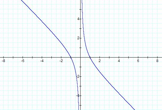
Here’s our first look at then equation. Do you have any conjectures and/or
assumptions based on the knowledge you’ve learned from Assignment 2?
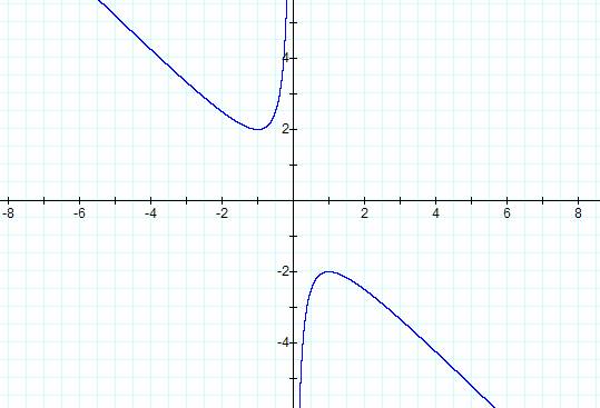
This new graph is very similar to our previous graphs but
at the same time it is also much different. First of all there are two different
parabolic shapes. In actuality these two curves are not parabolas. They are two
different parts of what is called a hyperbola. But we don’t want to discuss the
hyperbola yet. We’ll just concentrate on the different intersections. Secondly
they don’t seem to intersect the y axis at all. Since we have substituted b for
y we are now looking at the xb plane instead of the usual xy.
Now if we throw in some random value for b then we get a
line in the plane. Let’s say we want to graph b = 4. What happens?
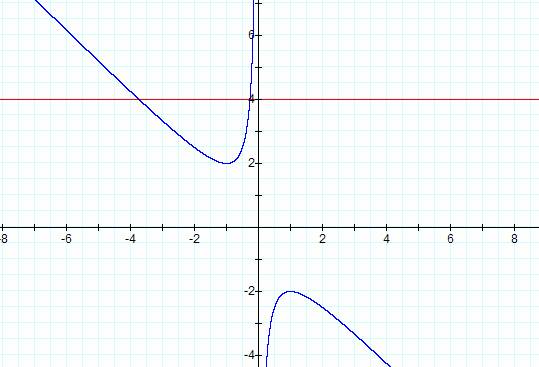
We produced a line running parallel to the x axis. And
notice that it intersects only one of our two curves. What does this mean?
These two intersections are known as the roots of our equation. We can also
guess from the picture that when b is equal to +/- 2 we will only get one
intersection. Let’s investigate this assumption. We’ll let b = +/- 2.
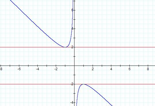
It looks like our two curves hit the lines in only one
place, namely +/- 2. So what does this mean and what happens if we have a value
between -2 and 2? Here’s the last graph on this investigation. We’ll let b = 1.
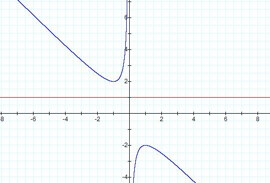
It turns out that this new line b = 1 does not interest
either of our curves. So we say that when we have an equation like ours then if
a line parallel to the x axis has a value of > 2 or < -2 we will have two
intersections. But if the line is equal to the absolute value of 2 then we’ll
only have one exact intersection and hence one root. Lastly if the line is
between 2 and -2 then we will have no intersections and no real roots.
Let’s shift our focus of our value of b and in turn look at
the values of c. Since we’ve exhausted the investigation of a in Assignment 2
and the values of b in the above discussion let’s complete the exploration with
c. We’ll keep the same equation as before and change the values of c, remember
that c was one in our original equation. Let’s start off by making c = 0.
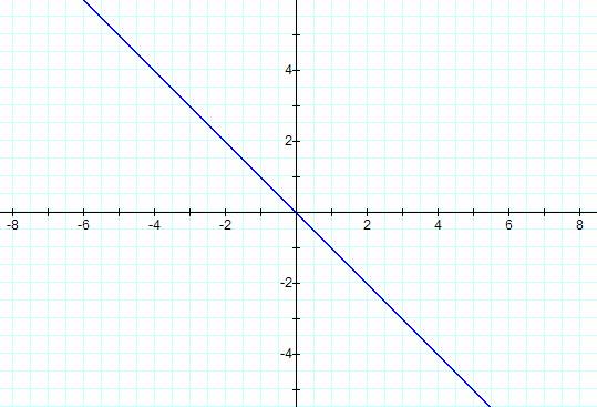
We get a straight line. Nothing too interesting here so
let’s suppose that c is a negative number. And if we remember correctly then we
know that in the original equation c was positive, hence 0 = ax2 +
bx + c. Let’s see what happens when c = -1.
This turns out to be extremely different from what we’ve
been working with for the last two exercises. Now we have what looks like a
rotation of 900 about the z axis. Here’s two 3d views of our graphs
so you can understand the rotation.
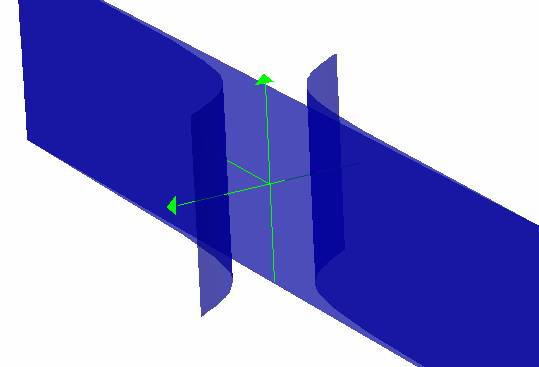
This is our new graph when c = a negative number
compared to our old graph below.
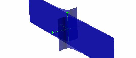
Can you tell a difference and see the rotation?
So in conclusion we’ve seen several interesting features of
our quadratic equation. If you have Graphing Calculator you can click on C Values to watch the c’s change and how it affects the
graph. But if you don’t then here’s what happens. When c is less than 0 you
will always have two roots for b. When c = 0 you will have exactly one root for
b. And when c is greater than 0 you will have the same case as above when some
places have two roots, two places has one root, and some places in the middle
have no real roots.
Write Up By David Drew